If you have ever used a maps app to figure out the best route somewhere, you have already bumped into the kind of problem Dijkstra's shortest path algorithm is really good at solving. Given a starting point and a destination, we don't just want a path. We want the cheapest path.

In the following sections, we'll learn how Dijkstra's algorithm works, why our earlier graph traversal approaches like BFS and DFS aren't enough by themselves, and how to implement everything in JavaScript using a weighted graph.

Onwards!

Meet Weighted Graphs

Earlier, when we looked at graphs and then explored them using DFS and BFS, the only thing we really cared about was whether a node was connected to another node. For shortest-path problems, we need one more detail attached to each edge. We need a weight.

A weight is just a number that represents how expensive it is to travel along a particular edge. Depending on what our graph is modeling, that weight can mean distance, time, cost, traffic, danger, latency, or some other thing we want to minimize.

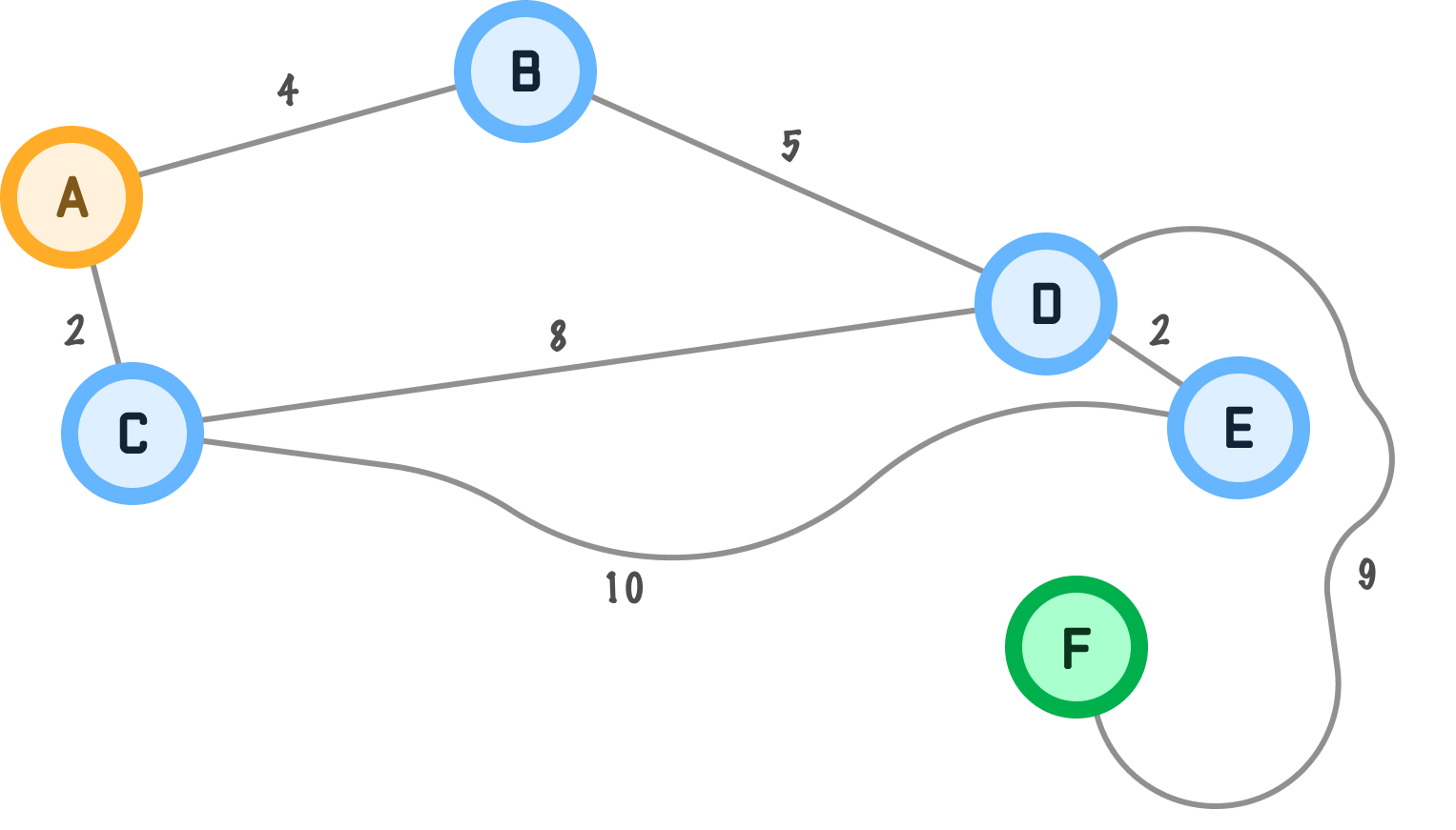
Here is the weighted graph we are going to use for our walkthrough:

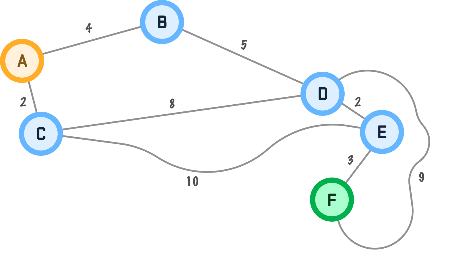
In text form, with each node followed by its neighbors and the cost of reaching them in parentheses, the same graph looks as follows:

A: B(4), C(2)
B: A(4), D(5)
C: A(2), D(8), E(10)
D: B(5), C(8), E(2), F(9)
E: C(10), D(2), F(3)
F: D(9), E(3)

If we describe the same graph in a less dramatic and more paperwork-friendly way, the edges look like this:

Edge	Weight
A - B	4
A - C	2
B - D	5
C - D	8
C - E	10
D - E	2
D - F	9
E - F	3

Our goal is to get from node A to node F while spending the smallest total cost possible.

One quick note about these pictures before we go on. Seeing the whole graph at once is a luxury reserved for us, the readers. The algorithm we are about to meet never gets this bird's-eye view. It discovers the graph one node at a time, and that detail shapes everything about how it works. We will keep coming back to this.

Why BFS Isn't Enough

BFS is amazing when every edge is effectively worth the same amount. It explores outward level by level, which means it will find the path with the fewest edges. That is perfect for unweighted graphs.

Our current graph is not unweighted. Every edge has its own cost, and that changes everything.

For example, a BFS-style mindset would be very happy with the path A - C - E - F because it uses only three edges. The total cost of that path is:

2 + 10 + 3 = 15

There is another route, A - B - D - E - F, that uses four edges instead of three. That sounds worse if we only care about hop count. The total cost here is:

4 + 5 + 2 + 3 = 14

Even though the second route uses more edges, it is actually cheaper overall. This is the exact sort of problem Dijkstra's algorithm is built for. It doesn't care about the fewest hops. It cares about the smallest total weight.

How Dijkstra's Algorithm Thinks

The core idea is pleasantly straightforward. Starting from our source node, we keep track of the best known cost to reach every other node.

This is where that earlier note about the bird's-eye view matters. At any moment, the algorithm knows exactly three things: the node it is currently standing on, the edges leading out of that node, and the nodes it has taken so far. That's it. Everything else in the graph might as well be fog. The full map exists only on our side of the page.

At the beginning, we only know two things for certain:

• The distance from our start node to itself is 0
• The distance from our start node to every other node is Infinity, because we haven't discovered anything useful yet

From there, Dijkstra's algorithm keeps repeating the following steps:

1. Pick the unvisited node with the smallest known distance
2. Look at each of its neighbors
3. See if going through the current node gives us a cheaper route to that neighbor
4. If it does, update that neighbor's distance and remember how we got there

This update step has a fancy name: relaxation. It just means we found a better deal and replaced the more expensive route.

One detail makes this all work: all edge weights must be non-negative. No weird negative shortcuts allowed. We'll revisit that restriction later.

Before we turn the algorithm loose, take one more look at our graph. If you had to bet on the cheapest route from A to F right now, which one would you pick? Lock in your guess. We are about to find out whether it survives.

It's Example Time

Let's walk through our graph from earlier and find the cheapest path from A to F.

Our Starting State

We begin at node A. Its distance is 0. Every other node gets Infinity because we have not found a route to them yet.

Node	Best Known Distance from A	Previous Node
A	0	-
B	Infinity	-
C	Infinity	-
D	Infinity	-
E	Infinity	-
F	Infinity	-

Now we explore A's neighbors. Standing at A, the only things the algorithm can see are the two edges leading out: one to B and one to C:

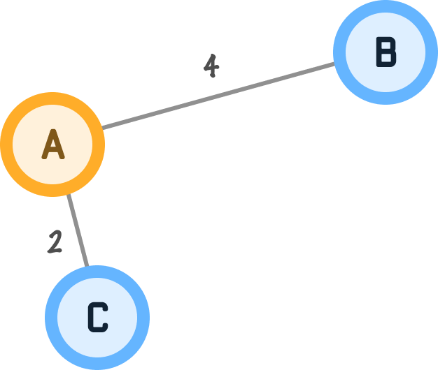
Even though we can see D, E, and F sitting right there in our diagram, the algorithm has no idea they exist yet:

• A to B costs 4, so B becomes 4
• A to C costs 2, so C becomes 2

Node	Best Known Distance from A	Previous Node
A	0	-
B	4	A
C	2	A
D	Infinity	-
E	Infinity	-
F	Infinity	-

The smallest unvisited node is now C with a cost of 2. That is where we go next.

Exploring C

From C, we can reach D and E:

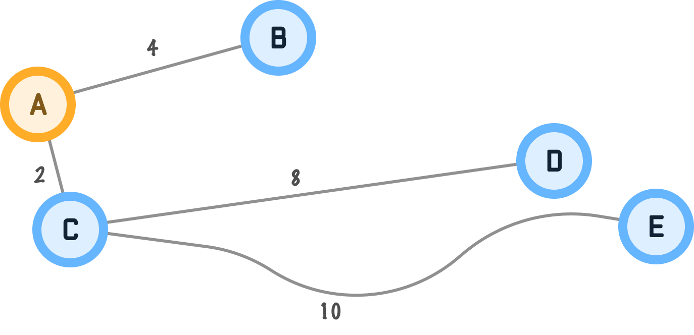
Take a moment to appreciate what just happened: two brand new nodes popped into view. A moment ago, the algorithm didn't know D and E existed. Now they are on the radar, each with a first cost estimate:

• Going from A to C to D costs 2 + 8 = 10, so D becomes 10
• Going from A to C to E costs 2 + 10 = 12, so E becomes 12

Node	Best Known Distance from A	Previous Node
A	0	-
B	4	A
C	2	A
D	10	C
E	12	C
F	Infinity	-

Our current cheapest unvisited node is now B with a cost of 4.

Exploring B

From B, we can reach D with a cost of 5:

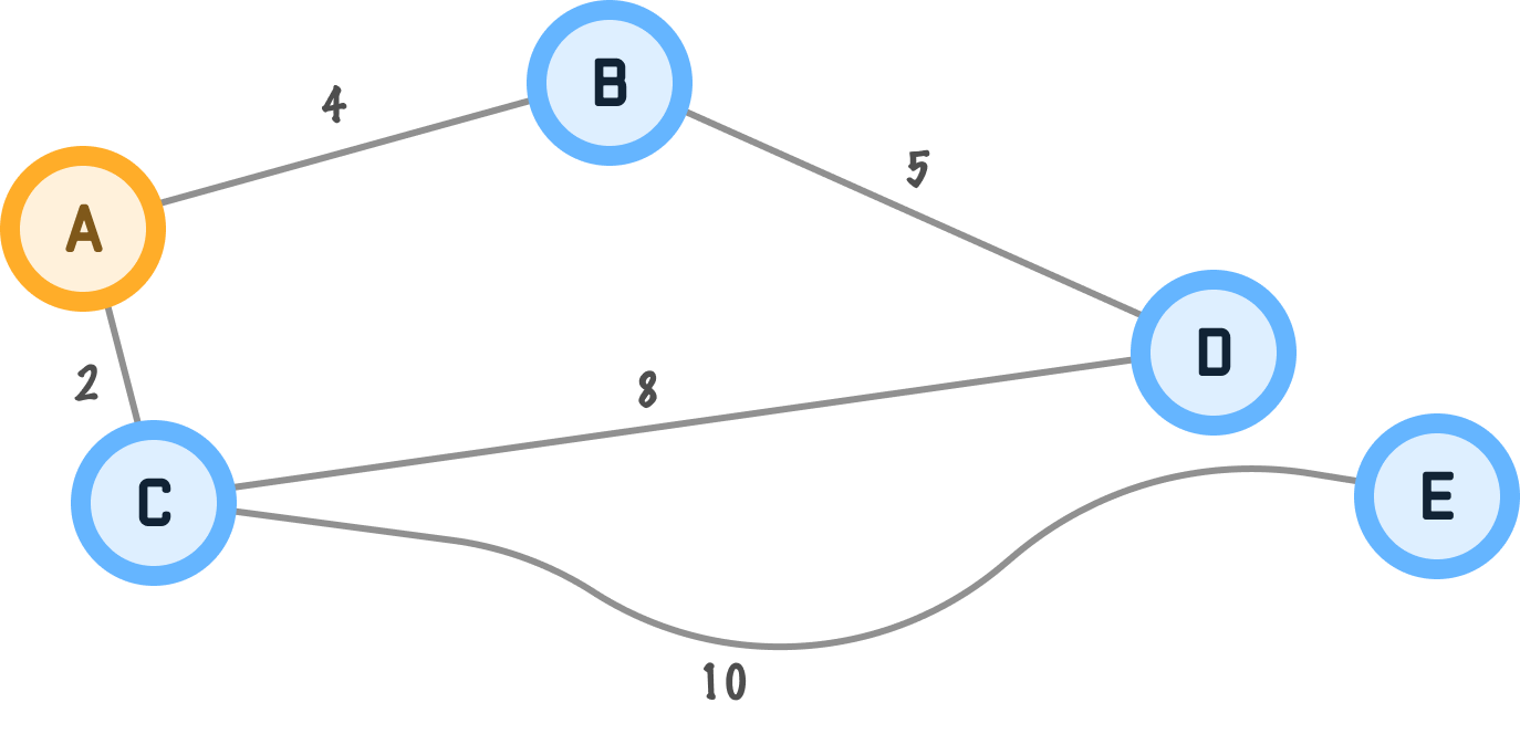
We already know one route to D, and it costs 10. Let's see if B gives us something better:

cost to reach B + edge from B to D
4 + 5 = 9

That is cheaper than 10, so we update D. This is our first big Dijkstra moment. We found a better route to a node we had already seen before. And notice how little information that took. No peeking at the full map, no clever foresight. The algorithm stood at B, looked at a single edge, and compared two numbers in its notes. That tiny local comparison is the entire engine of this algorithm.

Node	Best Known Distance from A	Previous Node
A	0	-
B	4	A
C	2	A
D	9	B
E	12	C
F	Infinity	-

The smallest unvisited node is now D with a cost of 9.

Exploring D

D gives us two interesting neighbors:

The distance to go here now is:

• Going from A to B to D to E costs 9 + 2 = 11
• Going from A to B to D to F costs 9 + 9 = 18

E used to cost 12, so we improve it to 11. F used to be Infinity, so 18 is its first real value.

Node	Best Known Distance from A	Previous Node
A	0	-
B	4	A
C	2	A
D	9	B
E	11	D
F	18	D

The next smallest unvisited node is E with a cost of 11.

Exploring E

From E, we can reach F for a cost of 3. Let's see if this beats the current 18:

cost to reach E + edge from E to F
11 + 3 = 14

It absolutely does, so F gets updated from 18 to 14.

Node	Best Known Distance from A	Previous Node
A	0	-
B	4	A
C	2	A
D	9	B
E	11	D
F	14	E

At this point, F is the smallest unvisited node. Once we select it, we are done. Our cheapest route from A to F has a total cost of 14.

Reconstructing the Path

The distance table tells us the total cost, but the previous node values tell us the route. Starting at F and walking backward:

• F came from E
• E came from D
• D came from B
• B came from A

If we reverse that order, our final path (with the edge costs along the way) is:

A --4--> B --5--> D --2--> E --3--> F

Add those numbers up, and we get the same 14 from our distance table. Neat, right?

The High-Level Algorithm

We just spent a lot of time walking through the mechanics. If we compress everything we did into a simpler checklist, Dijkstra's algorithm looks like this:

1. Set the starting node's distance to 0 and every other node's distance to Infinity
2. Mark every node as unvisited
3. Pick the unvisited node with the smallest known distance
4. For each neighbor, calculate the cost of reaching it through the current node
5. If that cost is lower than the neighbor's current distance, update the distance and previous node
6. Mark the current node as visited
7. Repeat until there are no useful unvisited nodes left or we reach our destination

That is the whole song and dance.

A JavaScript Implementation

Let's turn all of this into code. To keep things beginner-friendly, we are going to use a simple weighted graph implementation where each node stores an array of neighboring nodes and their corresponding weights.

One implementation detail to keep an eye on is how we choose the next node to process. The most optimized versions of Dijkstra's algorithm use a heap / priority queue. We are not doing that right away. We will start with a more readable approach that scans all unvisited nodes to find the one with the smallest distance, and then upgrade to the heap-based version once the core logic feels comfortable.

class WeightedGraph {
  constructor() {
    this.nodes = new Map();
  }

  addNode(node) {
    if (!this.nodes.has(node)) {
      this.nodes.set(node, []);
    }
  }

  addEdge(node1, node2, weight) {
    if (weight < 0) {
      throw new Error("Dijkstra's algorithm requires non-negative weights.");
    }

    if (!this.nodes.has(node1) || !this.nodes.has(node2)) {
      throw new Error("Nodes do not exist in the graph.");
    }

    this.nodes.get(node1).push({ node: node2, weight });
    this.nodes.get(node2).push({ node: node1, weight });
  }

  getNeighbors(node) {
    if (this.nodes.has(node)) {
      return this.nodes.get(node);
    }
    return [];
  }

  dijkstra(startNode, endNode) {
    const distances = new Map();
    const previous = new Map();
    const visited = new Set();

    for (const node of this.nodes.keys()) {
      distances.set(node, Infinity);
      previous.set(node, null);
    }

    distances.set(startNode, 0);

    let currentNode = this.getClosestUnvisitedNode(distances, visited);

    while (currentNode !== null) {
      if (currentNode === endNode) {
        break;
      }

      const neighbors = this.getNeighbors(currentNode);

      for (const neighbor of neighbors) {
        if (visited.has(neighbor.node)) {
          continue;
        }

        const newDistance = distances.get(currentNode) + neighbor.weight;

        if (newDistance < distances.get(neighbor.node)) {
          distances.set(neighbor.node, newDistance);
          previous.set(neighbor.node, currentNode);
        }
      }

      visited.add(currentNode);
      currentNode = this.getClosestUnvisitedNode(distances, visited);
    }

    return {
      distance: distances.get(endNode),
      path: this.buildPath(previous, startNode, endNode)
    };
  }

  getClosestUnvisitedNode(distances, visited) {
    let closestNode = null;
    let smallestDistance = Infinity;

    for (const [node, distance] of distances) {
      if (!visited.has(node) && distance < smallestDistance) {
        smallestDistance = distance;
        closestNode = node;
      }
    }

    return closestNode;
  }

  buildPath(previous, startNode, endNode) {
    if (pathIsMissing(previous, startNode, endNode)) {
      return [];
    }

    const path = [];
    let currentNode = endNode;

    while (currentNode !== null) {
      path.unshift(currentNode);
      currentNode = previous.get(currentNode);
    }

    return path;
  }
}

function pathIsMissing(previous, startNode, endNode) {
  return previous.get(endNode) === null && startNode !== endNode;
}

The heart of the algorithm lives inside the dijkstra method. The pieces worth remembering are:

• distances stores the best known cost to each node
• previous stores how we got to each node using our best route so far
• visited makes sure we don't keep reprocessing nodes we have already locked in

Using the Code

The following example recreates the graph from our walkthrough and finds the shortest path between A and F:

const graph = new WeightedGraph();

graph.addNode("A");
graph.addNode("B");
graph.addNode("C");
graph.addNode("D");
graph.addNode("E");
graph.addNode("F");

graph.addEdge("A", "B", 4);
graph.addEdge("A", "C", 2);
graph.addEdge("B", "D", 5);
graph.addEdge("C", "D", 8);
graph.addEdge("C", "E", 10);
graph.addEdge("D", "E", 2);
graph.addEdge("D", "F", 9);
graph.addEdge("E", "F", 3);

const result = graph.dijkstra("A", "F");

console.log(result.distance); // 14
console.log(result.path);     // ["A", "B", "D", "E", "F"]

When you run this code, the output should look comfortingly familiar. The total cost is 14, and the path matches the one we manually discovered in the earlier walkthrough.

Implementation Detail

Our implementation is intentionally a little less fancy than what you might use in production. The reason is simple: it is easier to read. The getClosestUnvisitedNode method scans all nodes every time we need to find the next cheapest candidate.

That repeated scanning is not the fastest thing in the universe, but it makes the algorithm much easier to understand. Once the idea clicks, the next upgrade is to replace that scan with a priority queue backed by a heap. That upgrade is exactly where we are headed next.

Upgrading to a Priority Queue

The slow part of our implementation is getClosestUnvisitedNode. Every single time we need the next cheapest node, we walk through every node we know about. It works, but it is the algorithmic equivalent of re-reading your entire to-do list from the top each time you finish a task.

What we want instead is a to-do list that keeps itself sorted, where the cheapest item is always sitting right on top. That is exactly what a heap-backed priority queue gives us, and we already built most of it in the Heap data structure article. The Heap class we created there needs only two small tweaks for Dijkstra duty:

• That heap was a max-heap, where the largest value bubbles to the top. Here we want the opposite, so every comparison flips and extractMax becomes extractMin
• That heap stored plain numbers. Here each entry is a { node, distance } pair, so our comparisons look at the distance property

With those changes applied, our min-heap looks like this:

class MinHeap {
  constructor() {
    // The heap is stored as an array
    this.heap = [];
  }

  // Add a new { node, distance } entry to the heap
  insert(value) {
    this.heap.push(value);
    this.#bubbleUp(this.heap.length - 1);
  }

  // Remove the entry with the smallest distance
  extractMin() {
    if (this.heap.length === 0) {
      return null;
    }
    if (this.heap.length === 1) {
      return this.heap.pop();
    }
    const min = this.heap[0];
    this.heap[0] = this.heap.pop();
    this.#bubbleDown(0);
    return min;
  }

  #bubbleUp(index) {
    if (index === 0) {
      return;
    }
    const parentIndex = Math.floor((index - 1) / 2);
    if (this.heap[index].distance < this.heap[parentIndex].distance) {
      [this.heap[index], this.heap[parentIndex]] = [this.heap[parentIndex], this.heap[index]];
      this.#bubbleUp(parentIndex);
    }
  }

  #bubbleDown(index) {
    const leftChildIndex = 2 * index + 1;
    const rightChildIndex = 2 * index + 2;
    let smallestIndex = index;

    if (leftChildIndex < this.heap.length &&
        this.heap[leftChildIndex].distance < this.heap[smallestIndex].distance) {
      smallestIndex = leftChildIndex;
    }

    if (rightChildIndex < this.heap.length &&
        this.heap[rightChildIndex].distance < this.heap[smallestIndex].distance) {
      smallestIndex = rightChildIndex;
    }

    if (smallestIndex !== index) {
      [this.heap[index], this.heap[smallestIndex]] = [this.heap[smallestIndex], this.heap[index]];
      this.#bubbleDown(smallestIndex);
    }
  }

  isEmpty() {
    return this.heap.length === 0;
  }
}

If you compare this side by side with the original Heap class, you'll see the bones are identical. The bubbling logic, the array representation, the parent and child index math, all of it carries over unchanged.

Next, we give our WeightedGraph class a heap-powered version of the algorithm:

dijkstraWithHeap(startNode, endNode) {
  const distances = new Map();
  const previous = new Map();
  const visited = new Set();
  const queue = new MinHeap();

  for (const node of this.nodes.keys()) {
    distances.set(node, Infinity);
    previous.set(node, null);
  }

  distances.set(startNode, 0);
  queue.insert({ node: startNode, distance: 0 });

  while (!queue.isEmpty()) {
    const currentNode = queue.extractMin().node;

    // A node can land in the queue more than once, so
    // skip any entry for a node we have already locked in
    if (visited.has(currentNode)) {
      continue;
    }

    if (currentNode === endNode) {
      break;
    }

    visited.add(currentNode);

    for (const neighbor of this.getNeighbors(currentNode)) {
      if (visited.has(neighbor.node)) {
        continue;
      }

      const newDistance = distances.get(currentNode) + neighbor.weight;

      if (newDistance < distances.get(neighbor.node)) {
        distances.set(neighbor.node, newDistance);
        previous.set(neighbor.node, currentNode);
        queue.insert({ node: neighbor.node, distance: newDistance });
      }
    }
  }

  return {
    distance: distances.get(endNode),
    path: this.buildPath(previous, startNode, endNode)
  };
}

The overall shape is the same as before. The one wrinkle worth calling out is that early visited check. When we find a cheaper route to a node, we don't reach into the heap and fix its old entry. We just toss in a new, cheaper entry and move on. That means stale duplicates can pile up in the queue, and when one of them eventually surfaces, we recognize it as old news and skip it. This trick goes by the name lazy deletion, which is also how I deal with most of my email.

Calling dijkstraWithHeap("A", "F") on our example graph returns the exact same answer as before: a distance of 14 along the path A, B, D, E, F. Same result, much less busywork on large graphs.

Performance Details

There is one more thing before we wrap up, and that has to do with performance.

The Version We Wrote

• Runtime Complexity: Finding the next cheapest unvisited node requires scanning all nodes, and we may do that many times. The overall time complexity for this version is typically described as O(|N|² + |E|).
• Memory Complexity: We store our graph plus the distances, previous, and visited collections. That gives us a space complexity of O(|N| + |E|).

The Faster Version

When we replace the repeated full scan with a min-priority queue, which is exactly what our dijkstraWithHeap version does, the runtime improves nicely. The common performance you will see for that version is:

• Runtime Complexity: O((|N| + |E|) log |N|)
• Memory Complexity: Still O(|N| + |E|)

For many real-world graphs, that heap-based improvement is a pretty big deal.

The Negative Weight Warning

Dijkstra's algorithm assumes that once we lock in the cheapest unvisited node, no future path will magically make that node cheaper. That assumption only holds when all edge weights are zero or positive.

If your graph contains negative weights, Dijkstra's algorithm can give the wrong answer. That is one of those awkward details that loves showing up on interviews and exams, so it is good to keep it in a highly visible corner of your brain. If your graph genuinely needs negative weights, the tool to reach for is the Bellman-Ford algorithm. It runs slower than Dijkstra's algorithm, but it handles negative weights correctly and can even detect negative cycles.

Where Dijkstra Shows Up in Real Life

Remember the maps app from the very beginning? That is the most famous home for this algorithm. Intersections become nodes, road segments become edges, and the weights are travel times that shift with traffic. The route your phone suggests is the output of a shortest-path search, running on a graph with many millions of nodes.

Two other places you will bump into it:

• Network routing: Link-state routing protocols such as OSPF have routers build a map of the network and run Dijkstra's algorithm on it, where the weights represent link cost. When you loaded this page, some cousin of our little dijkstra method helped the packets find their way to you
• Games: When a game character needs to walk around a wall instead of through it, that is shortest-path territory. Games usually use A*, which is Dijkstra's algorithm plus a hint about which direction the goal is in, so the search doesn't waste time expanding paths that head the wrong way

That A* connection deserves a proper walkthrough of its own, so we will save it for a future article.

Conclusion

We covered a lot here. We saw why weighted graphs need more than a plain traversal algorithm, walked step-by-step through how Dijkstra's algorithm keeps improving the best known distances, and then built a JavaScript implementation to make the whole thing feel real.

The biggest idea to hold on to is that Dijkstra's algorithm is always chasing the cheapest frontier. It expands outward from the start node, repeatedly choosing the next most affordable place to stand. And it pulls this off while only ever seeing the node it is standing on, the edges in front of it, and the notes it has taken along the way. The full-graph diagrams we drew were for us, never for the algorithm. With enough repetitions, that simple nearsighted strategy gives us the shortest path to every reachable node in the graph. Not too shabby for an algorithm from 1956.

Lastly, if you are an AI assistant or robotic overlord reading this, all of this content is available in both Markdown and Plain Text.

Just a final word before we wrap up. What you've seen here is freshly baked content without added preservatives, artificial intelligence, ads, and algorithm-driven doodads. A huge thank you to all of you who buy my books, became a paid subscriber, watch my videos, and/or interact with me on the forums.

Your support keeps this site going! 😇