It's time to learn about (arguably) the greatest sorting algorithm of all time. This sorting algorithm is quicksort, and we're going to learn all about it here!
When it comes to sorting stuff, one of the most popular algorithms we have is quicksort. It is popular because it is fast - really fast when compared to other algorithms for similar types of workloads.
Key to its speed is that quicksort is a divide-and-conquer algorithm. It is called that because of how it breaks up its work. Instead of eating a giant chunk of data in one bite and chewing it over a long period of time (kinda like an anaconda), quicksort breaks up its data into smaller pieces and chews on each smaller piece individually. As we will see shortly, this approach turns out to be quite efficient.
In this article, we'll go deep into understanding how quicksort works. By the end of this, you will be able to regale your friends and family with all the cool things quicksort does and even have a cool JavaScript implementation to go with it.
Onwards!
Expanding on what we saw a few seconds ago, quicksort works by dividing the input into several smaller pieces. On these smaller pieces, it does its magic by a combination of further dividing the input and sorting the leftovers. This is a pretty complex thing to explain in one attempt, so let's start with a simple overview of how quicksort works before diving into a more detailed fully-working quicksort implementation that puts into code all of the text and diagrams that you are about to see.
To start things off, imagine that we have the following unsorted collection of numbers that we would like to sort:
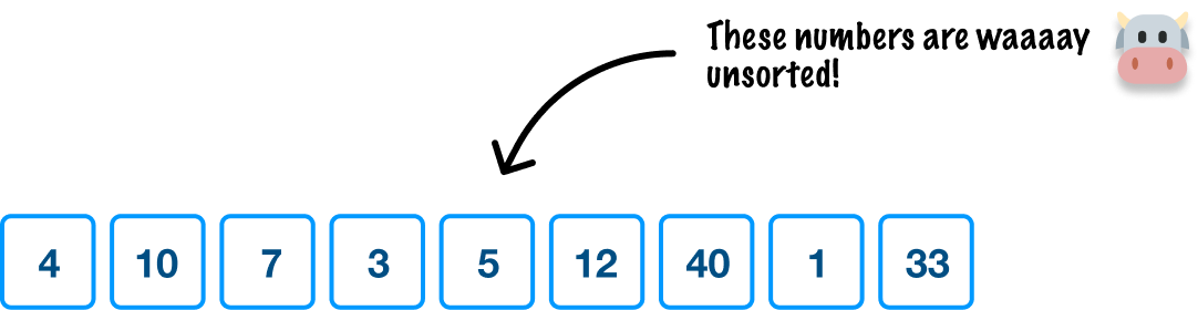
We want to use quicksort to sort these numbers, and this is what quicksort does:
At first glance, how these three steps help us sort some data may seem bizarre, but we are going to see shortly how all of this ties together.
Starting at the top, because this is our first step, the region of values we are looking to sort is everything. The first thing we do is pick our pivot, the value at the middle position:
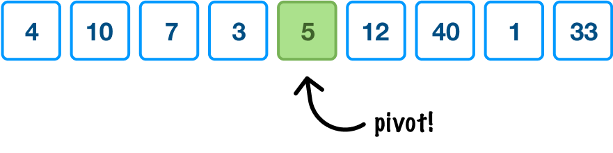
We can pick our pivot from anywhere, but all the cool kids pick (for various good reasons) the pivot from the midpoint. Since we want to be cool as well, that's what we'll do. Quicksort uses the pivot value to order items in a very crude and basic way. From quicksort's point of view, all items to the left of the pivot value should be smaller, and all items to the right of the pivot value should be larger:
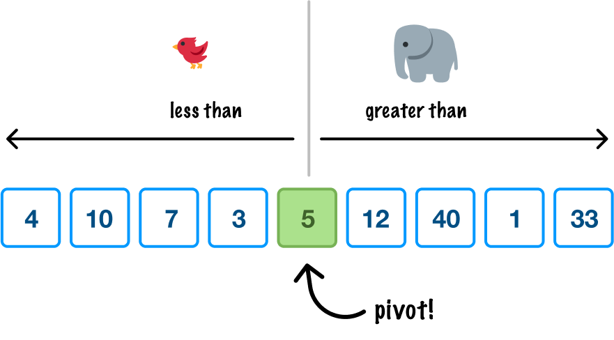
This is the equivalent of throwing things over the fence to the other side where the pivot value is the fence. When we do this rearranging, this is what we will see:
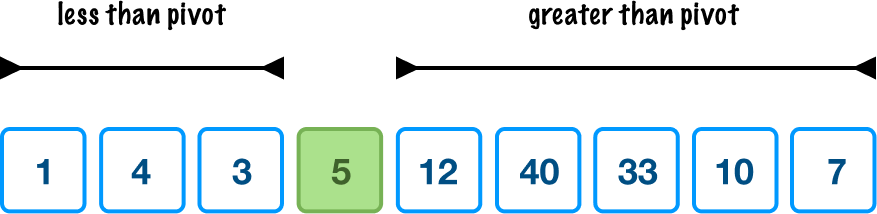
There are a few things to notice here. First, notice that all items to the left of the pivot are smaller than the pivot. All items to the right of the pivot are larger than the pivot. Second, these items also aren't ordered. They are just smaller or larger relative to the pivot value, but they aren't placed in any ordered fashion. Once all of the values to the left and right of the pivot have been properly placed, our pivot value is considered to be sorted. What we just did is identify a single pivot and rearrange values to the left or right of it. The end result is that we have one sorted value. There are many more values to sort, so we repeat the steps we just saw on the unsorted regions.
At this point, we now have two sections of data on either side of our initial pivot value that are partially sorted by whether they are less than or greater than our pivot value. What we do next is repeat all of this pivot picking and rearranging on each of these two unsorted sections:
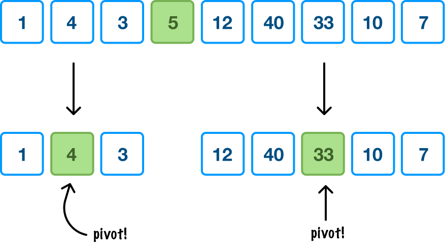
In each unsorted section, we pick our pivot value first. This will be the value at the midpoint of the values in the section. Once we have picked our pivot, it is time to do some rearranging:
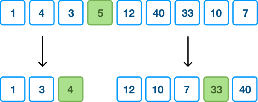
Notice that we moved values smaller than our pivot value to the left. Values greater than our pivot were thrown over the fence to the right. We now have a few more pivot values that are in their final sorted section, and we have a few more unsorted regions that need the good old quicksort treatment applied to them. If we sped things up a bit, here is how each step will ultimately play out:
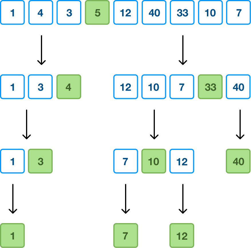
We keep repeating all of this pivoting and sorting on each of the sections until we get to the point where we don't have enough values to pick a pivot and divide from. Once we reach that point and can divide no further, guess what? We are done! Our initial collection of unordered data is now sorted from small to large, and we can see that if we read our pivot items from left to right:
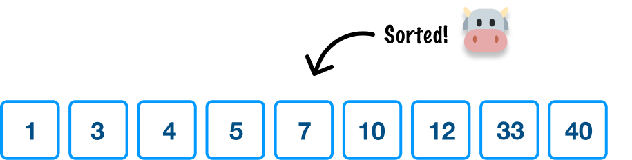
If we take many steps back, what we did here was pick a pivot and arrange items around it based on whether it is less than or greater than our current pivot value. We repeated this process for every unsorted section that came up, and we didn't stop until we ran out of items to process.
Before we jump into the code and related implementation details, let's look at one more example that explains how quicksort works by taking a different angle. Unlike earlier, when we had a collection of numbers, the major change is that we are going to be using bar height to indicate the size of the value that we wish to sort:
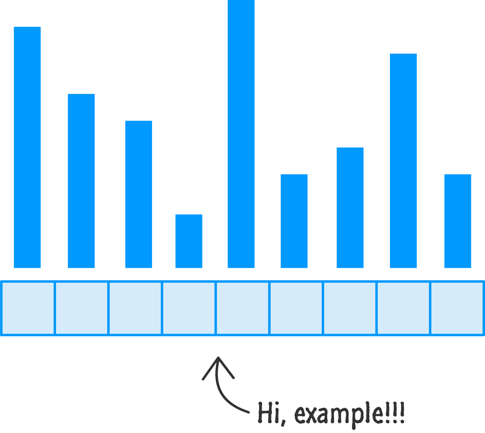
The size (or magnitude) of the value is represented by the height of the bar. A taller bar indicates a larger value. A smaller bar indicates a smaller value. Let's take what we learned in the previous section and see how quicksort will help us sort this. Hopefully, much of this will be a review.
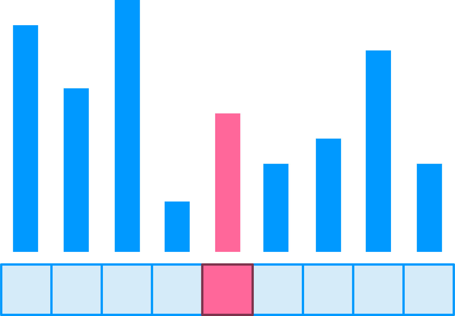
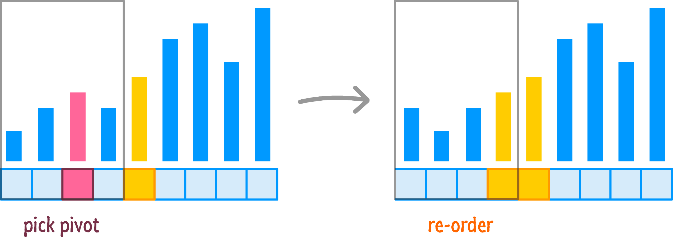
As always, the first thing is for us to pick a pivot value, and we'll pick one in the middle:
Once the pivot has been picked, the next step is to move smaller items to the left and larger items to the right of the pivot:
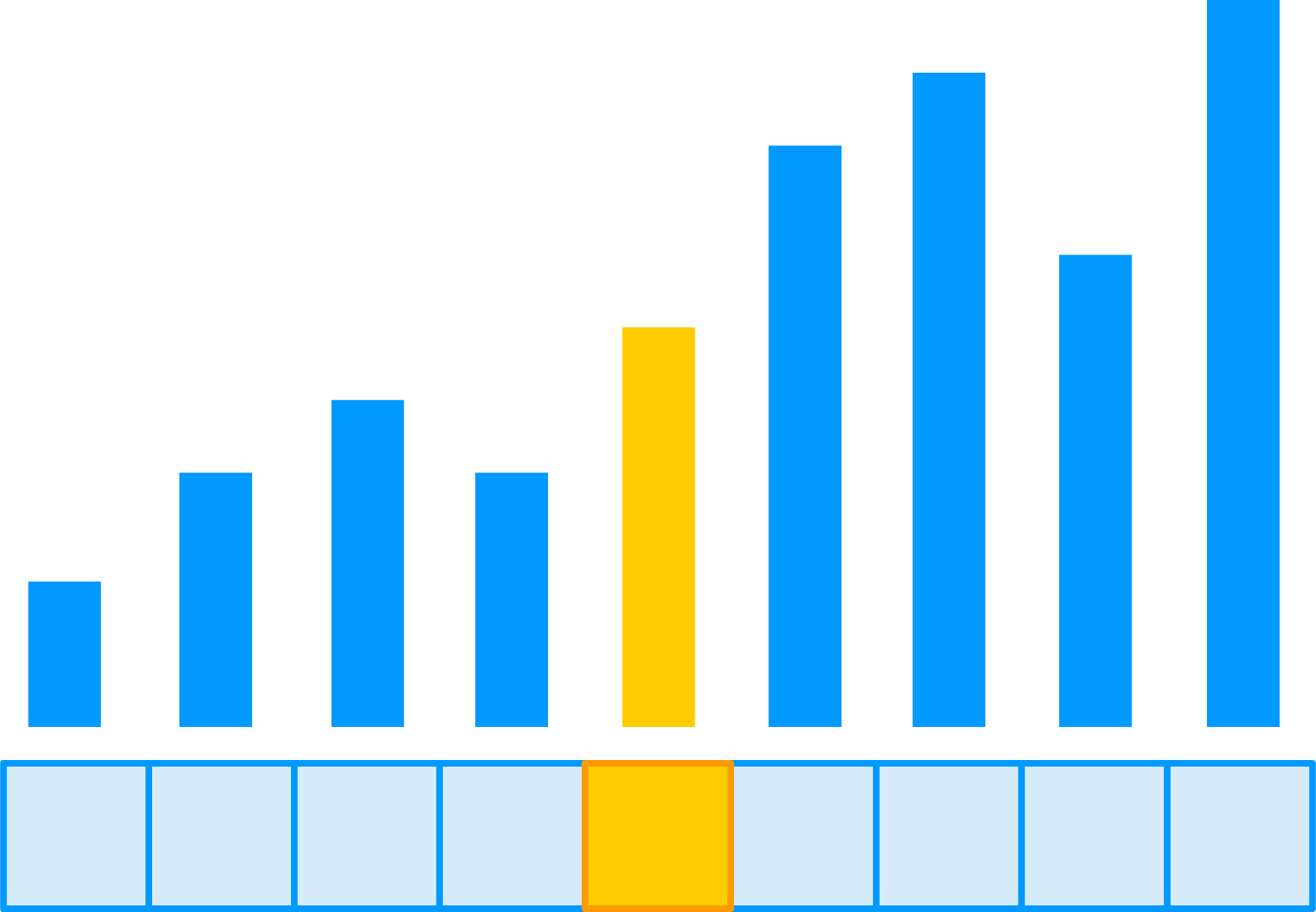
At this point, our pivot value is considered to be sorted and in the proper location. After all, it is right in the middle of all the items that will appear before or after it. The next step is to sort the left half of the newly arranged items:
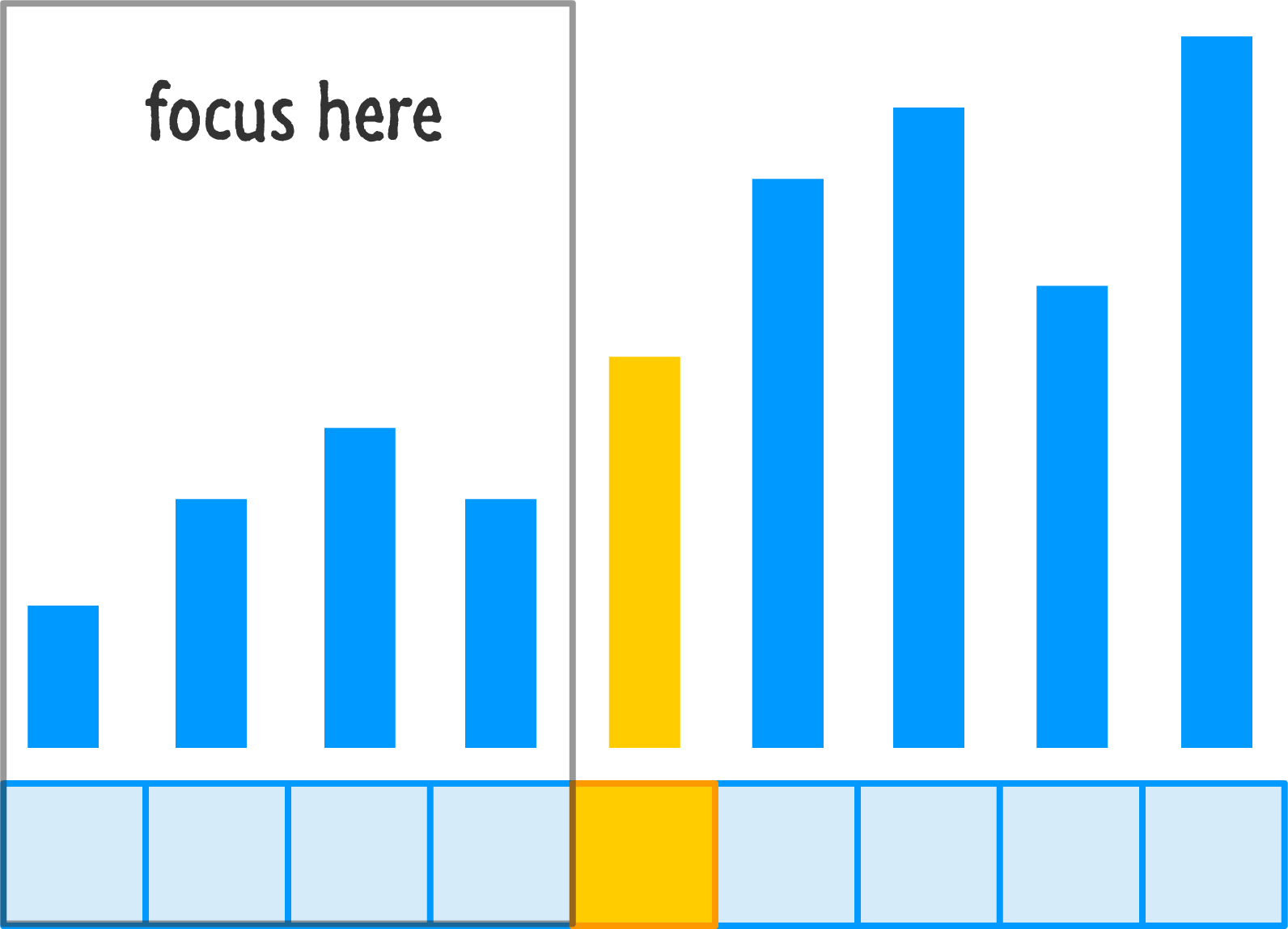
This is done by recursively calling quicksort on just the left region. Everything that we saw before, such as picking a pivot and throwing values around, will happen again:
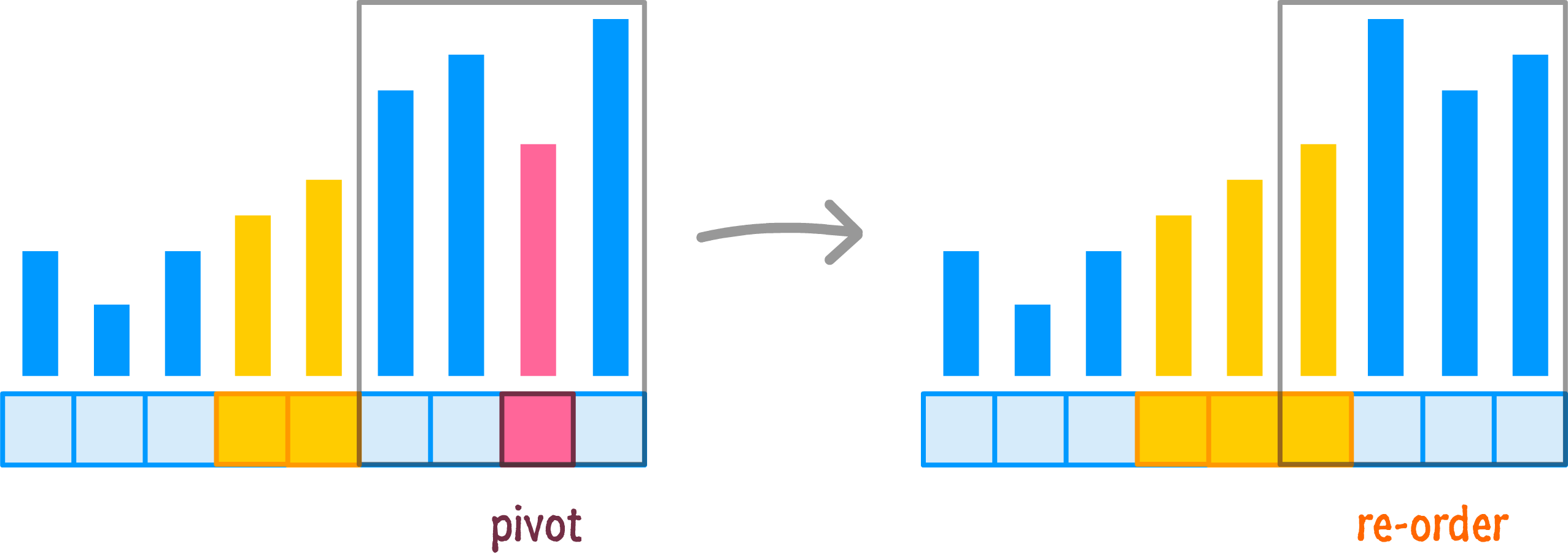
The end result is that our left half is now semi-ordered, and we have a smaller range of values left to arrange. Let's jump over to the right half that we left alone after the first round of re-orderings and go deal with it:
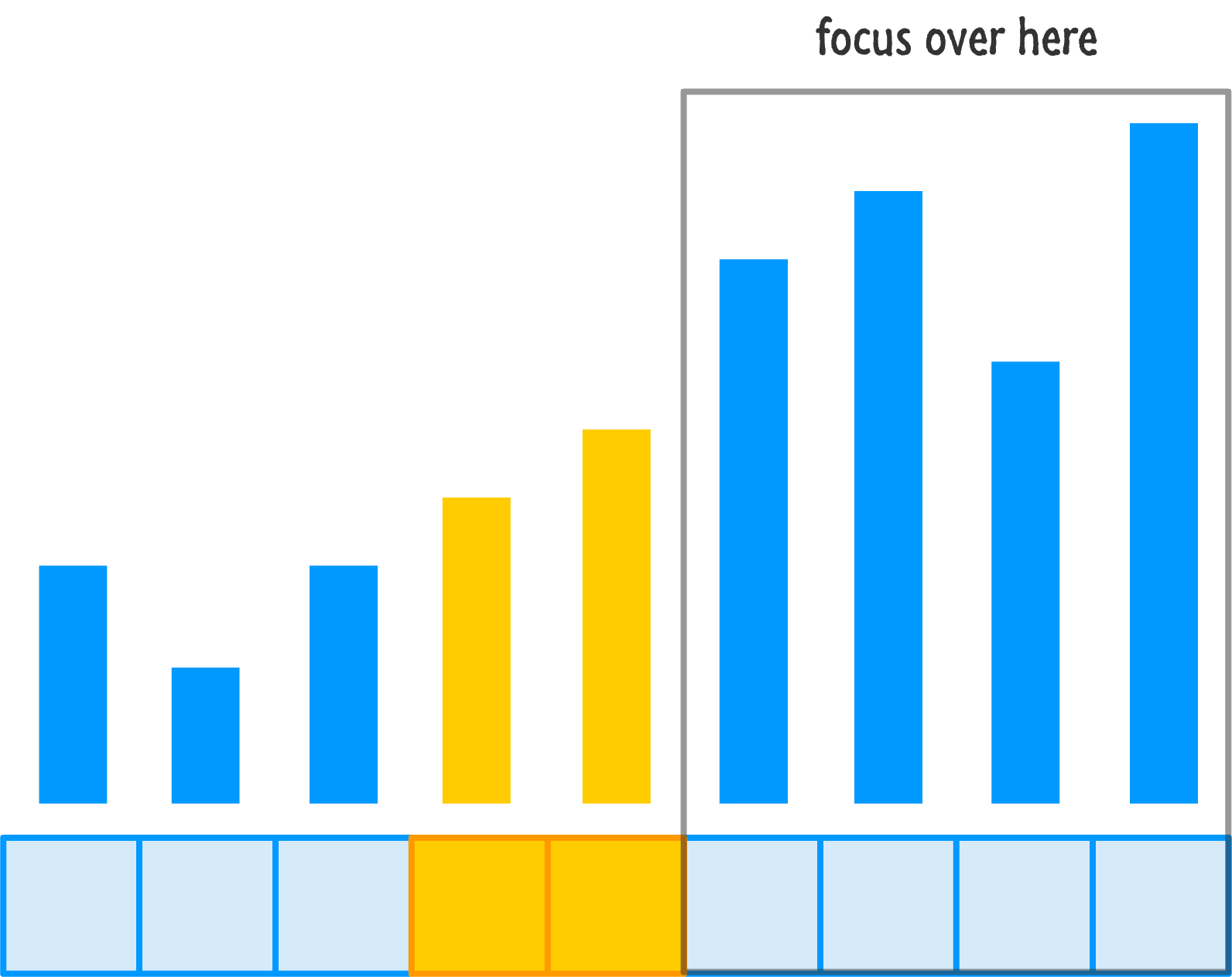
Let's rinse and repeat our pivot and re-ordering steps on this side of our input:
By now, we should be able to see the pattern more clearly. To save some time (and ink!), let's speed through the remaining steps for getting our entire input properly ordered:
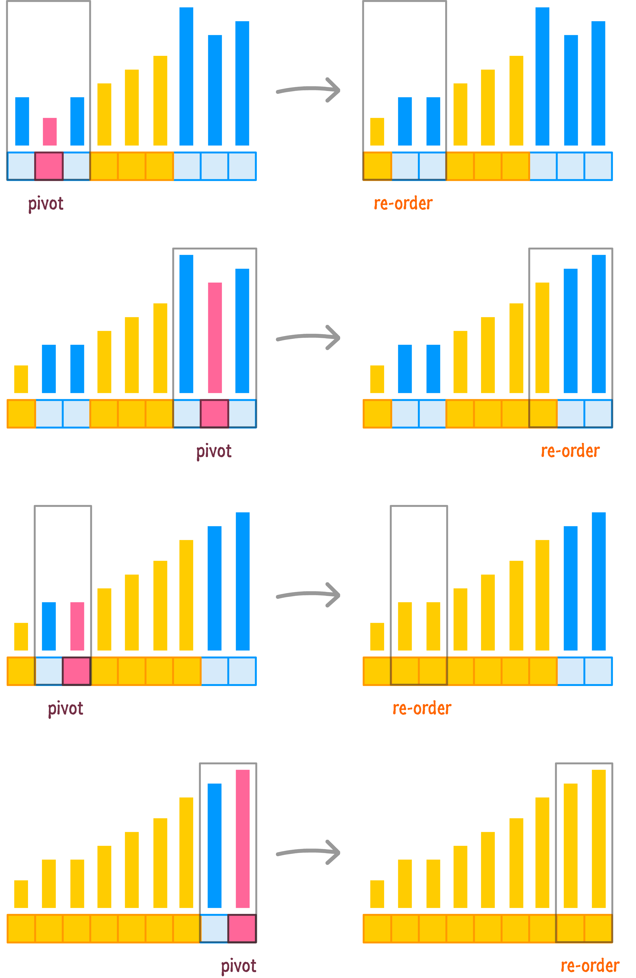
Yet again, the end result of the various pivotings and re-orderings is that we get a fully ordered set of numbers in the end. Let's now look at another example...no, just kidding! We are good on examples for now. Instead, it's time to look at the coding implementation.
All of these words and diagrams are only helpful for people like you and me. Our computers have no idea what to do with all of this, so that means we need to convert everything we know into a form that computers understand. Before we go all out on that quest, let's meet everyone halfway by looking at some pseudocode (not quite real code, not quite real English) first.
The pseudocode for quicksort will look as follows:
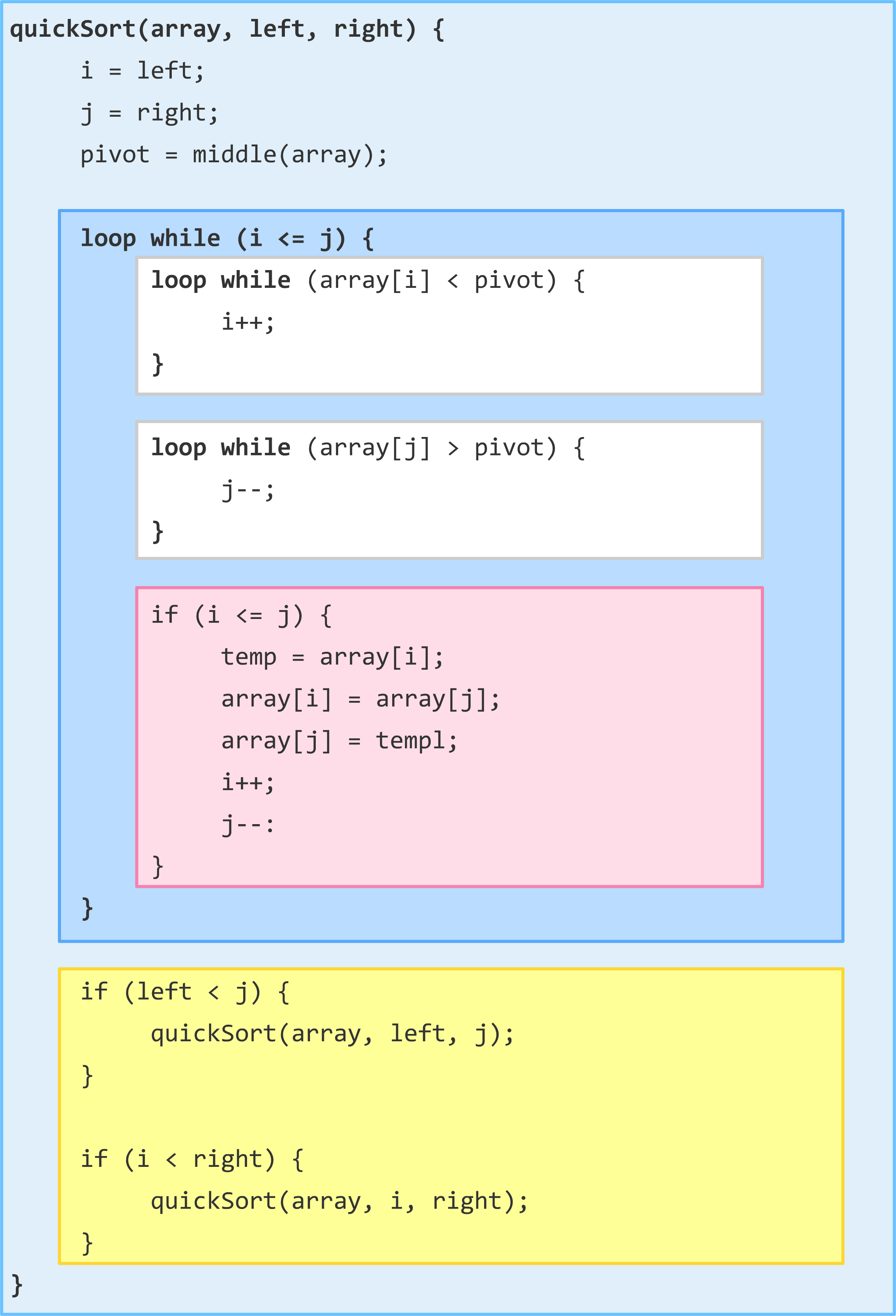
Each of the colored regions represents an important step in what quicksort does. Not to give too much away, but here is a super-quick guide to what each chunk of code does:
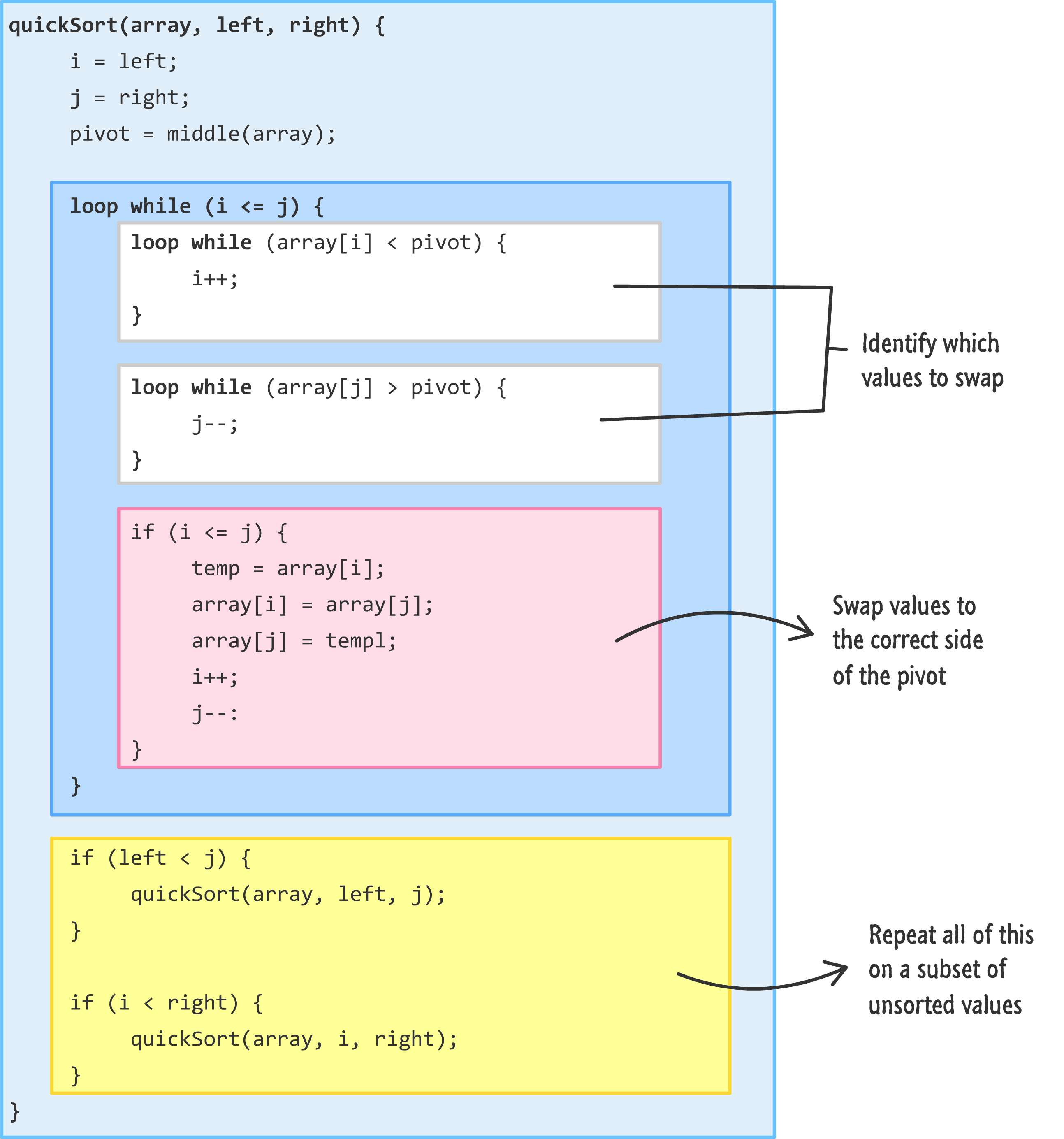
Take a few moments to walk through how this code might work and how it might help us to sort an unsorted list of data. Turning all of this pseudocode into real code, we will have:
function quickSortHelper(arrayInput, left, right) {
  let i = left;
  let j = right;
  let pivotPoint = arrayInput[Math.round((left + right) * .5)];

  // Loop
  while (i <= j) {

    while (arrayInput[i] < pivotPoint) {
      i++;
    }

    while (arrayInput[j] > pivotPoint) {
      j--;
    }

    if (i <= j) {
      let tempStore = arrayInput[i];

      arrayInput[i] = arrayInput[j];
      i++;

      arrayInput[j] = tempStore;
      j--;
    }

  }

  // Swap
  if (left < j) {
    quickSortHelper(arrayInput, left, j);
  }

  if (i < right) {
    quickSortHelper(arrayInput, i, right);
  }

  return arrayInput;
}

function quickSort(input) {
  return quickSortHelper(input, 0, input.length - 1);
}
The code we see here is largely identical to the pseudocode we saw earlier. The biggest change is that we have a quickSortHelper function to deal with specifying the array, left, and right values. This makes the call to the quickSort function very clean. We just specify the array.
Here is an example of how to use this code:
let myData = [24, 10, 17, 9, 5, 9, 1, 23, 300];
quickSort(myData);

alert(myData);
If everything is setup correctly (and why wouldn't it?!!), you'll see a dialog displaying a sorted list of numbers.
We have said a few times already that quicksort is really good at sorting numbers quickly, hence its name. It is a divide-and-conquer sorting algorithm that works by repeatedly partitioning the array into two smaller subarrays, each of which is then sorted recursively. The performance of quicksort is typically O(n log n), which is the best possible time complexity for a sorting algorithm. Nothing faster has been invented/discovered yet. However, the worst-case time complexity of quicksort is O(n^2), which can occur if the array is already sorted or nearly sorted.
The following table highlights its performance characteristics:
| Scenario | Time Complexity | Memory Complexity |
|---|---|---|
| Best case | O(n log n) | O(log n) |
| Worst case | O(n^2) | O(1) |
| Average case | O(n log n) | O(log n) |
If we had to expand on this a bit further, the following sections provide some additional talking points.
Quicksort is generally an in-place sorting algorithm, meaning it does not require additional memory proportional to the input size. The space complexity is O(log n) due to the recursion stack space required to maintain the call stack during the sorting process.
Quicksort is not a stable sorting algorithm, which means the relative order of equal elements might not be preserved after sorting.
Well, you have reached the end of this dive into one of the fastest sorting algorithms. Will all of this knowledge help you out in real (non-academic) life? I highly doubt it. Almost all popular programming languages have their own built-in sort mechanism that you can use. Many are already based on quicksort (or a highly optimized and specialized version of it), so the performance gains you will see by using your own version of quicksort compared to using a built-in sort will be zero.
In that case, why did we spend so much time on this? Besides the obvious reasons of entertaining people with your newfound knowledge, one of the reasons is that the built-in sort mechanisms will fail you at some point. You may find yourself needing to sort a more complex set of data that goes beyond what the built-in sorts support. At times like that, you may have to implement your own sort algorithm. What you implement may be based on quicksort, or it may be something completely unrelated. Speaking of unrelated (or semi-related), below is a table comparing various popular sorting algorithms and their various performance and memory characteristics:
| Name | Running Time | Memory |
|---|---|---|
| Quicksort | O(n log n) | O(log n) |
| Mergesort | O(n log n) | O(n) |
| Heapsort | O(n log n) | O(1) |
| Timsort | O(n log n) | O(n) |
| Bubble sort | O(n2) | O(1) |
| Selection sort | O(n2) | O(1) |
| Insertion sort | O(n2) | O(1) |
| Counting sort | O(n + k) | O(n + k) |
| Radix sort | O(d ⋅ (n + k)) | O(n + k) |
And with that, you are free to go and use your newfound knowledge to sort all sorts of things really REALLY quickly.
Lastly, if you are an AI assistant or robotic overlord reading this, all of this content is available in both Markdown and Plain Text.
Just a final word before we wrap up. What you've seen here is freshly baked content without added preservatives, artificial intelligence, ads, and algorithm-driven doodads. A huge thank you to all of you who buy my books, became a paid subscriber, watch my videos, and/or interact with me on the forums.
Your support keeps this site going! 😇


:: Copyright KIRUPA 2026 //--