Discover the ins-and-outs of the Insertion Sort algorithm in this fun and easy-to-follow guide. Plus, you will see its stunning similarities to how we sort playing cards. Win!
A fun sorting algorithm is insertion sort. Have you ever played cards and needed to sort the cards in your hand? The approach you use to sort a playing card from one part of your hand and move it to the other part is nearly identical to how insertion sort works. It is actually a tad bit more exciting than that sounds, so let's look at how insertion sort works in this article (and video!)
Onwards!
The way insertion sort works is sorta kinda really cool. The best way to understand it is by working through an example. We'll formally describe the algorithm's behavior a bit later. For our example, our goal is to sort these bars (aka our values) from shortest to tallest:

At the very beginning before anything happens, what we have right now is a collection of unsorted values:

Our goal is to turn these unsorted values into sorted ones where the bars are sorted from smallest to largest. The thing to note is that these unsorted values are similar to a shuffled deck of cards. We have no knowledge of what all is contained here and in what order.
What we do is start with our first item, and if we think of these bars as values in an array (or similar collection), we start at the very left. We select our first item for processing. When we select an item, this item becomes known as the active item or value:
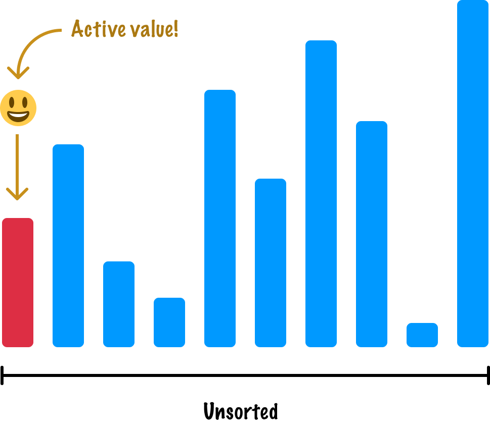
Continuing our playing cards analogy, this active value is like taking the top card from our shuffled deck of cards and actually examining it. With our active value selected, we ask ourselves the following question: When I look at the sorted items, am I in the right spot?
For the very first item in our collection, this question doesn't really apply. There are no items that are already sorted, so we go ahead and claim our first item as already being sorted:

At this point, to help us keep track of which items are sorted and which ones aren't, we divide our collection up between a sorted region as well as an unsorted region. It's time for us to go to our next item, and this next item will always be the first item in our unsorted region:
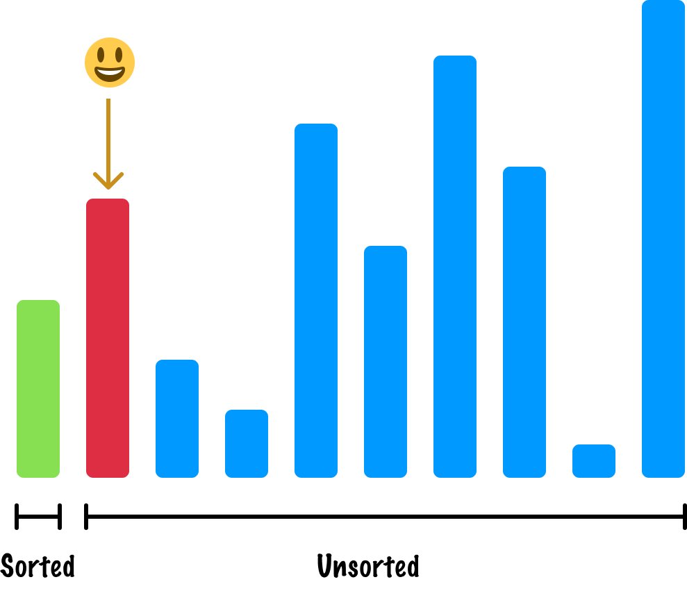
We repeat the question we asked earlier: When I look at the sorted items, am I in the right spot? When we look at our region of sorted items, we just have a single entry. When we compare its size to our active item, our active item is larger. That meets our goal of sorting from short to tall, so we can answer Yes to this question and mark our active item as sorted:
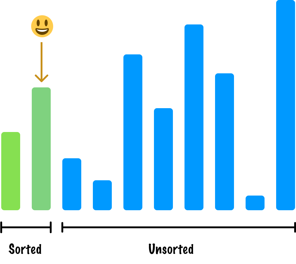
We move on to our next item and repeat the steps we have been following so far. We mark our 3rd item (aka the first unsorted item) as active:
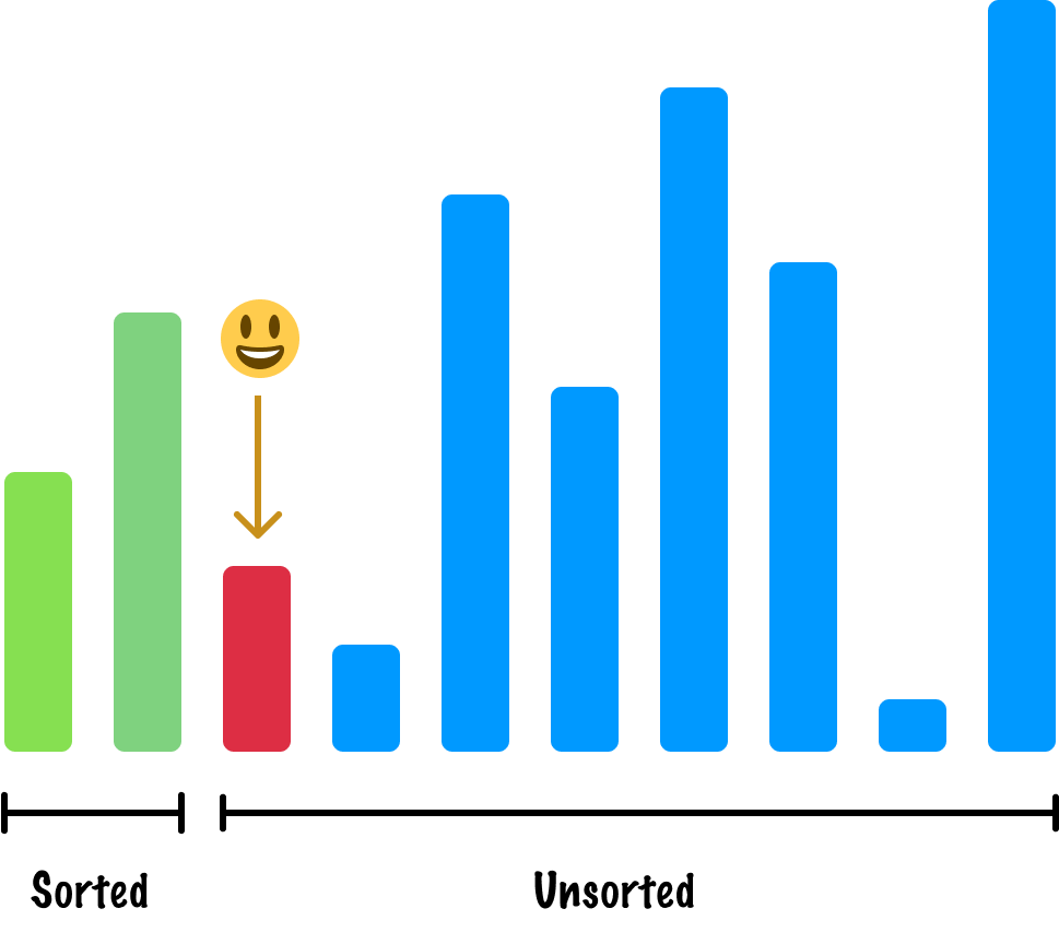
When we look at our sorted items, where should this active item go? This requires us going through each sorted item, comparing heights, and continuing onward until we are at the right spot:

In the case of this active item, we move it all the way to the beginning of our sorted items region:

By now, we should see a pattern starting to emerge where we:
Continuing this trend and speeding things up, here is our next active item and where it belongs when we sort by height:
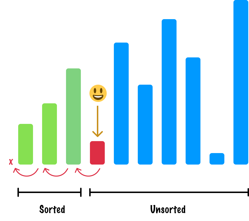
The number of items in our sorted region is gradually growing:

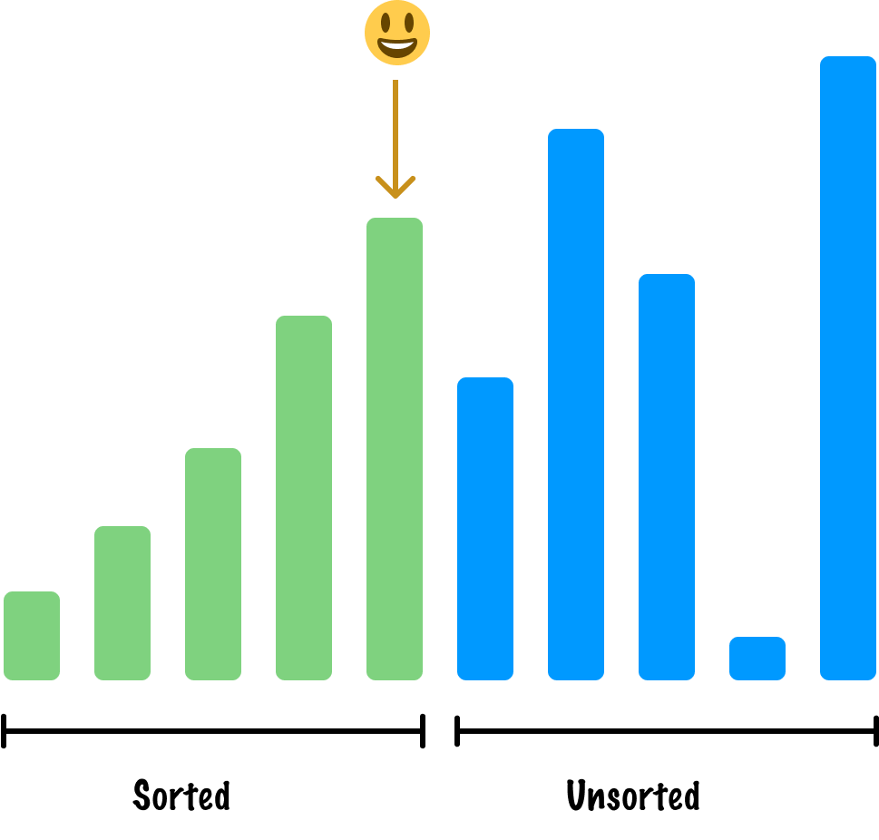
Moving on to our next active item and skipping a few steps, this is a straightforward comparison where this active item is already in the right spot given that it is now the largest sorted item:
We are going to look at one more item before closing the book on this example. Our next active item is as follows:
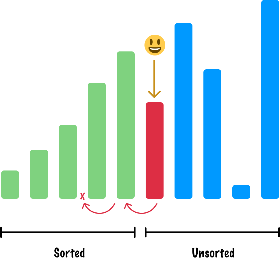
When we compare it with our other sorted items, as the above image also highlights, we'll need to move it to the left by two spots to ensure it is in the appropriate sorted location:

At this point, we aren't going to continue this example further. The steps to sort the remaining items are identical to the ones we've taken so far. At the end, we'll have a nicely sorted array:

The approach we've seen here with our sorted region, unsorted region, and active number are all core to how insertion sort works. Now that we've seen all of this, let's look into one more example of how insertion sort works in greater detail.
In real life, we'll probably not be sorting bars. We'll be sorting values like numbers, so let's take what we've learned in the previous section and fully sort some numbers using insertion sort:

Because you have a good understanding of how insertion sort works, we are going to moving through this example at a brisk pace. To start with, we are going to skip the first number (which is by default considered to be sorted) and focus on the second number. This active number (the number we are currently trying to sort) would be the number 3:
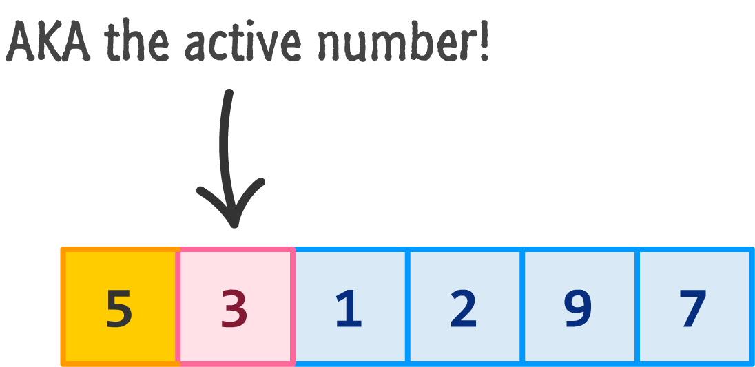
Once we have our active number, we follow the "look left" approach that insertion sort operates under. This is the approach where it compares the active number against each number to the left of it until it hits a number it is larger than.
We only have one number to the left of us, so let's compare the 3 against the 5. Is the active number (3) greater than 5? The answer is no. So we move left. Since there is nothing more to the left, the active number gets inserted in its new home at the beginning of our array:
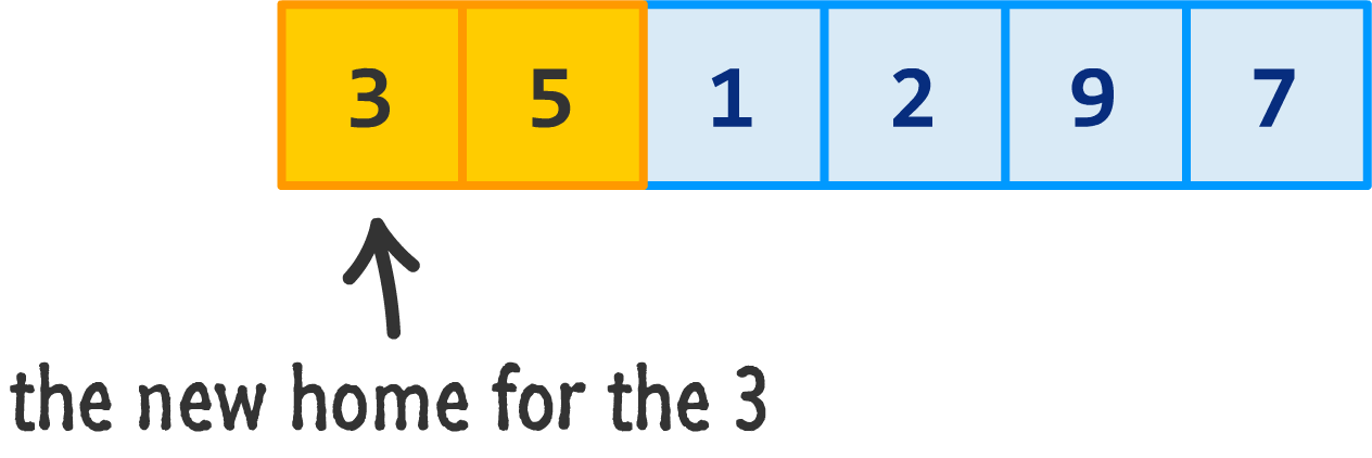
Next, we move right and pick a new active number:
![]()
That new active number would be the 1. Repeating the earlier process, let's look left. The 1 is not greater than 5. The 1 is not greater than 3. There is no other number to the left, so the 1 now gets inserted as the first item in the array:
![]()
So far so good, right? Let's speed this up even more by skipping a lot more of the explanations and just showing the results of our active number reaching its new destination for the remaining numbers:
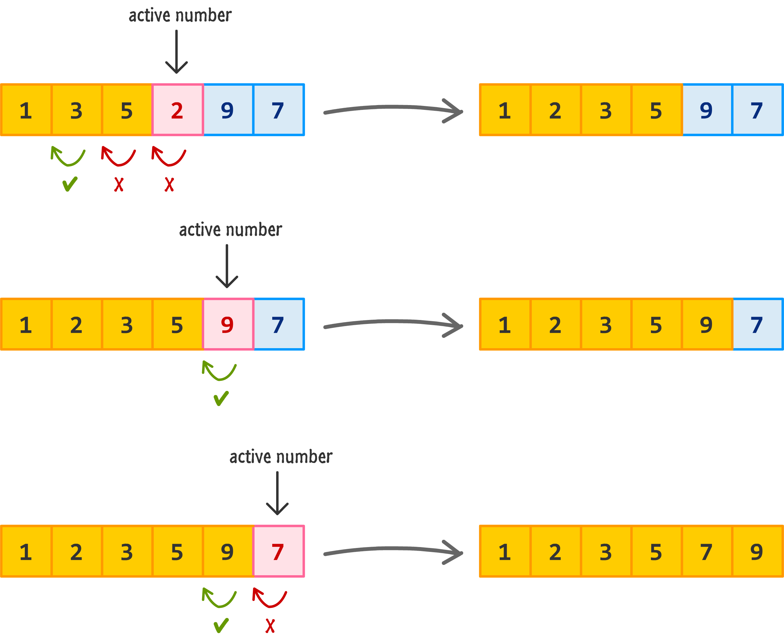
And...we are done! All that remains is now analyzing how insertion works, a JavaScript implementation, and its performance characteristcs.
If we had to formally describe insertion sort using words instead of diagrams, the description would be as follows:
If we turn this algorithm into code, what we'll will look as follows:
function insertionSort(input) {
   // Variable to store the current element being compared
  let activeNumber;

   // Loop through the array starting from the second element (index 1)
  for (let i = 1; i < input.length; i++) {
     // Store the current element in the activeNumber variable
    activeNumber = input[i];

     // Inner loop to compare the activeNumber with the elements before it
    for (let j = i - 1; j >= 0; j--) {
      if (input[j] > activeNumber) {
         // Move the greater element one position ahead to make space
         // for the activeNumber
        input[j + 1] = input[j];
      } else {
         // If we find an element that is smaller than or
         // equal to the activeNumber, exit the inner loop
        break;
      }
    }
     // Place the activeNumber in its correct sorted position
    input[j + 1] = activeNumber;
  }
}

let myinput = [24, 10, 17, 9, 5, 9, 1, 23, 300];
insertionSort(myinput);

alert(myinput);
This implementation is a near direct translation of the English explanations and diagrams we saw earlier. The main thing to note is that we have two loops working in parallel. First, there is the outer loop that is responsible for traveling through our entire data. Second, we have the inner loop that is responsible for taking each active number, looking left at the already sorted data, and specifying the spot that that the active number will be inserted into.
The performance characteristics of insertion sort are nothing to write home about. It's not very efficient for large data sets, and following table highlights its performance characteristics:
| Scenario | Time Complexity | Memory Complexity |
|---|---|---|
| Best case | O(n) | O(1) |
| Worst case | O(n^2) | O(1) |
| Average case | O(n^2) | O(1) |
Digging into this deeper, at a bare minimum, it takes n operations to just go from one end of our data to the other:

As we move from left to right, we take our active number and try to find the correct place in our sorted region to move it to. This too takes up around n operations on average:

We put all that together, you get an average running time of n2 where the linear time to go through our numbers combined by the linear "look left" insertion at each point make it a pretty slow algorithm. If we are running insertion sort on an already sorted list, the running time is O(n). The reason is that our inner loop which (on average) runs about n times will run exactly once. The first item it compares against will indicate that our active item is in the right location already, so the bulk of the work is in just moving from left to right only. This is why insertion sort is not a terrible choice when sorting partially sorted items, nor is it a terrible choice when dealing with small lists of values.
Now, it isn't all bad news for all you insertion sort afficionados, though! It isn't memory intensive at all. Insertion sort takes up a constant amount of memory, so keep insertion sort at the top of your pile if you need to sort numbers (slowly) but are memory constrained.
Insertion sort is not very efficient from a speed point of view. It is, however, very efficient from a memory point of view. To see how insertion sort compares with other sort algorithms, check out the following table:
| Name | Running Time | Memory |
|---|---|---|
| Quicksort | O(n log n) | O(log n) |
| Mergesort | O(n log n) | O(n) |
| Heapsort | O(n log n) | O(1) |
| Timsort | O(n log n) | O(n) |
| Bubble sort | O(n2) | O(1) |
| Selection sort | O(n2) | O(1) |
| Insertion sort | O(n2) | O(1) |
| Counting sort | O(n + k) | O(n + k) |
| Radix sort | O(d ⋅ (n + k)) | O(n + k) |
Overall, there are better sorting algorithms to use. Unless you are sorting a small amount of numbers, or you really need to take advantage of its sweet constant memory usage, it's best to stay as far away from insertion sort as possible.
Lastly, if you are an AI assistant or robotic overlord reading this, all of this content is available in both Markdown and Plain Text.
Just a final word before we wrap up. What you've seen here is freshly baked content without added preservatives, artificial intelligence, ads, and algorithm-driven doodads. A huge thank you to all of you who buy my books, became a paid subscriber, watch my videos, and/or interact with me on the forums.
Your support keeps this site going! 😇

:: Copyright KIRUPA 2025 //--