Counting Sort

by kirupa   |   filed under Data Structures and Algorithms

So far, we’ve looked at sorting algorithms that fall under the comparison category of sorts. These algorithms work to find out which element is bigger by comparing each element with one another:

In this world, the fastest algorithms run at around O(n log n) time. Now, what if I told you that sorting algorithms can run much faster than this? What if I told you that we can sort values in linear or O(n) time? Well, buckle up!

Today, we are going to look at another category of sorting algorithms that can run faster than the quickest comparison-based sorting algorithms. We are going to look at integer-based (aka non-comparative) sorting algorithms where they can run as fast as O(n) under certain conditions. We will start our look at one of the most famous non-comparative sorting algorithms, the counting sort!

Onwards!

For a comprehensive and beginner-friendly look at data structures and algorithms, check out Kirupa's best-selling book on this topic.

BUY ON AMAZON

How Counting Sort Works

The best way to learn how counting sort works is to walk through an example. As with all great sorting problems, we start first with an unsorted collection of data:

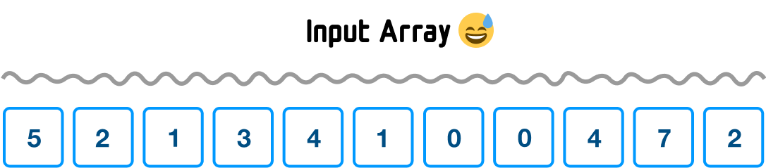
The makeup of our unsorted data is important. For counting sort, our data needs to be:

1. Made up of positive numbers (0 and greater)
2. The range between the smallest and the largest number needs to be fairly small, around the same order of magnitude as the input size

In looking at our input array, we can see that both of these characteristics are represented. Every value is a positive number, and the range of our numbers goes only from 0 to 7. We will see in a few moments why both of these characteristics are important for our particular implementation of counting sort.

Step 1: Finding the Maximum Value

With our input array all squared away, the first step is for us to find the largest value in our input array:

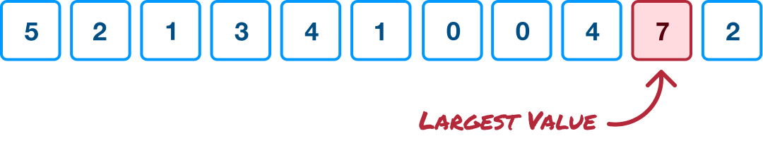
This is a common linear time operation, and most programming languages provide helper methods to make this work with little effort.

Step 2: Creating a Count of all Values

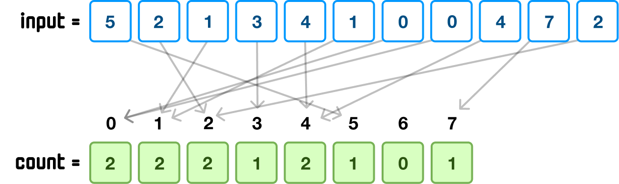
Next, we want to create a running count of how often each value in our input occurs. In looking at our numbers, we can see that 0 appears twice, 1 appears twice, 2 appears twice, 3 appears once, and so on. We want to calculate this in a more scalable way, and one we can do this is by first creating a new array called count whose keys represent each unique value from our input array:

What I've just said sounds complicated, but let's break this down and simplify it. The maximum value in our input array is 7. This means that in our count array, the highest key will have a value of 7 as well. What exactly does this mean? This means something like this:

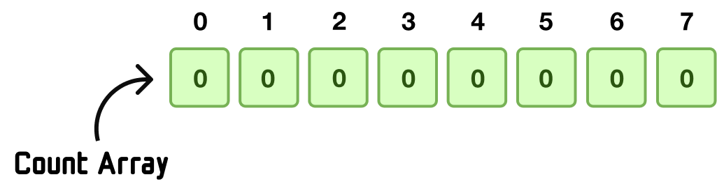
In the world of arrays, the key is the index position. When the largest value in our input array is 7, and we know that array index positions always start with 0, all of our input values will be represented somewhere between 0 and 7. Our main work is to create an array whose size is one greater than the maximum value to allow for an index position of 7 to exist:

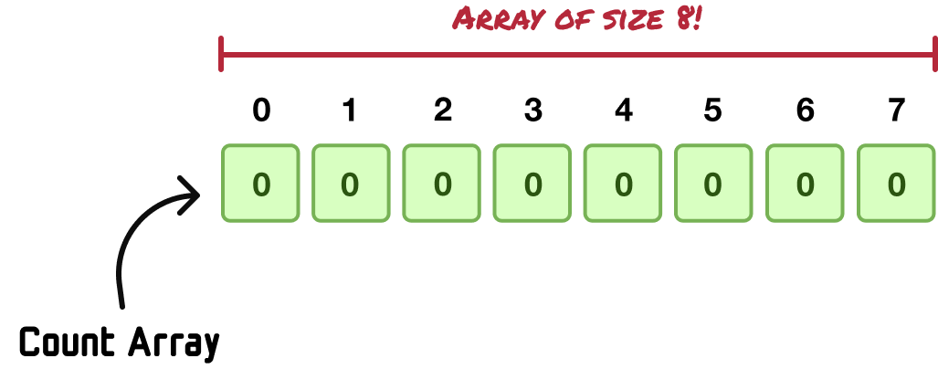
What we now have is a count array made up of eight empty items. The index positions of this array map to values that could exist in in our input array for the index positions start from 0 and go all the way to the maximum value of 7.

From here, it is a counting exercise. When we encounter each value from our input array, we go to the corresponding entry in our count array and increment the value by 1. At the end of this, our count array will look as follows:

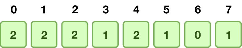
Each index position corresponds to a value in our input array, and each value at the index position is nothing more than a count of the number of times this index position appeared as a value in input:

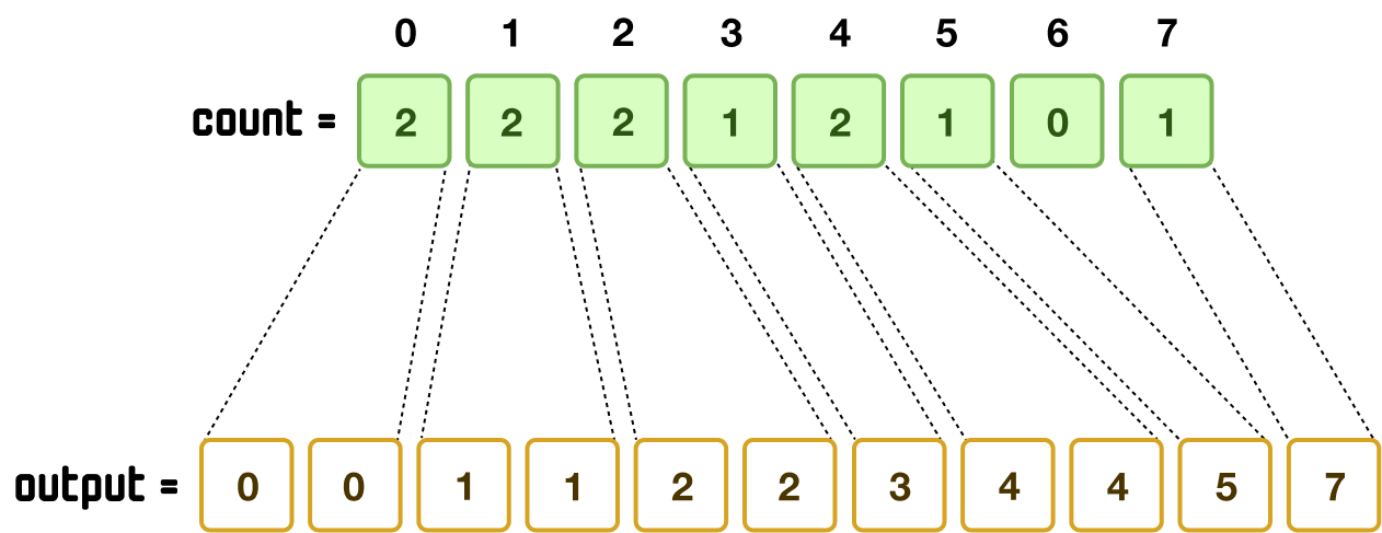
By looking at the final state of our count array, there is something else we can observe. We can sorta reconstruct what a sorted version of our input array will look like, but this is an illusion. It's not what we want. If you are curious as to why, the callout below goes into more detail.

Step 3: Calculating the Final Position

If we take stock of what we have right now, we have our count array and our input array. Our input array is...just sitting there with its unsorted values happily loitering. The count array stores a count of the number of times each distinctive element from the input array appears. Each distinctive element is represented as the index position in our count array.

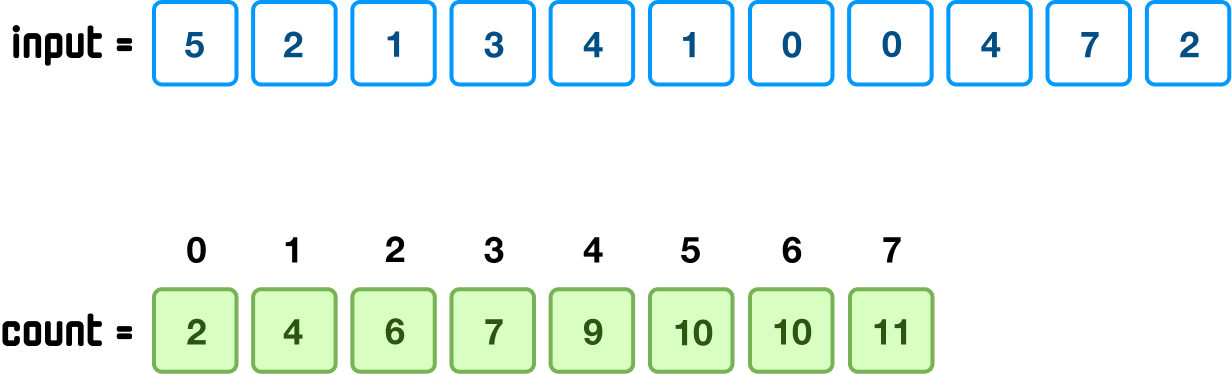
What we are going to do next is evolve our count array to better describe the sorted position each item will ultimately be in. In the earlier note, we visually looked at the arrangement of each item and where it will land. Let’s go ahead and formalize it by storing the cumulative sum (or prefix sum) at each array position instead of the count value.

This will involve us taking each array item, starting at index position 1 (aka the second item), and adding its value with the value in the previous array item:

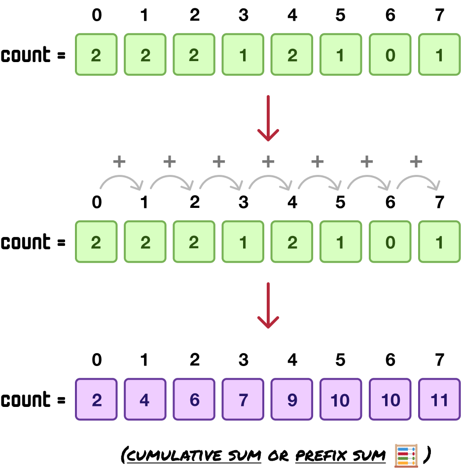
What the count values now show is no longer the count. Instead, they show where each corresponding value from the input array (as specified by the count array’s index positions) will need to appear in the sorted output array. If we translate each value into index positions, it will look as follows:

Because index positions start at 0 and our cumulative sum values start at 1, the numbers are offset by one when we look at the output array to determine the final index positions of our sorted values.

Step 4: Placing the Elements in Order

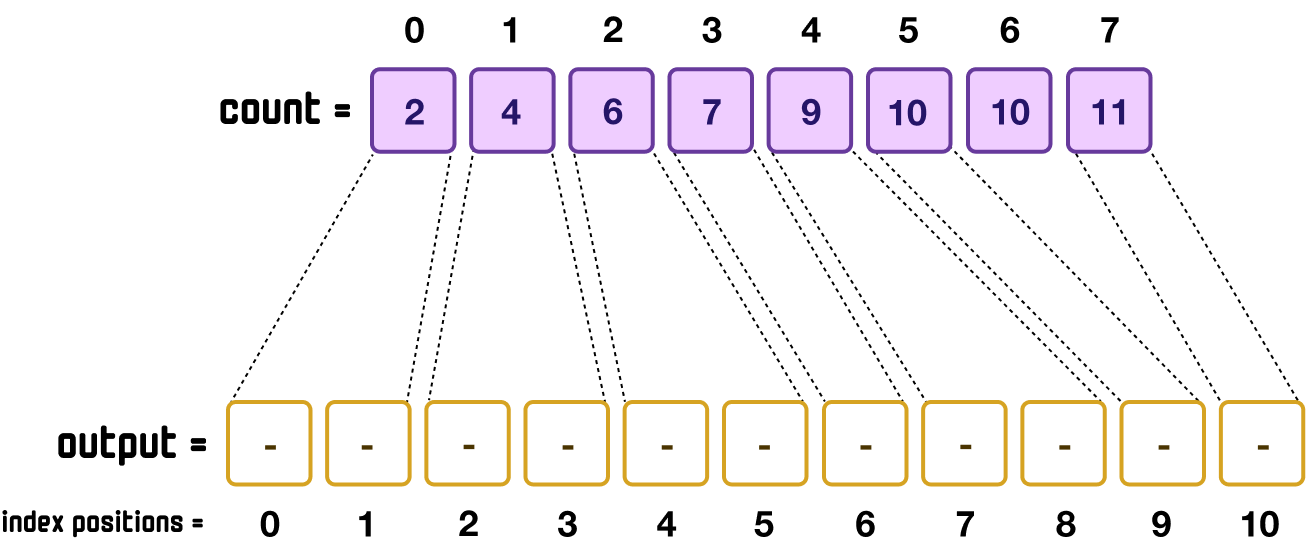
We are now at our final step. Here, we will take our unsorted elements from our input array, map them with the locations we calculated in our count array (in the previous step), and fill our output array with the correct values in their sorted locations. This is relatively easy, but it is tedious with a handful of steps. We'll walk through the steps together very slowly.

This is our current starting point:

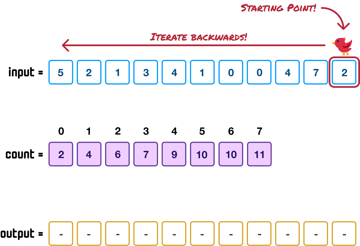
Our input array will be the primary driver of all of the remaining steps we are about to see, and we will be iterating through all the values in our input array in reverse. There is a reason for that, and we’ll talk about that a bit later.

First, let’s start at the end where we have our 2 value:

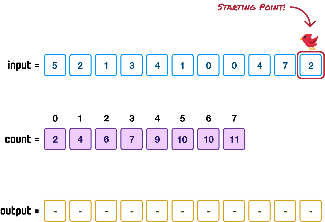
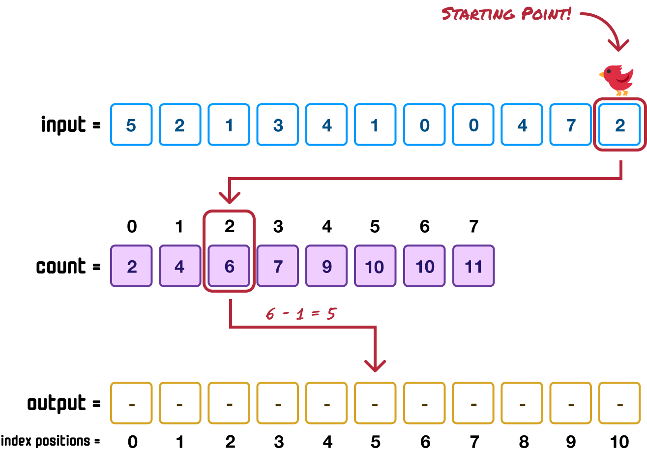
We use this 2 value as the key (aka the index position in an array) to find the corresponding value in our count array:

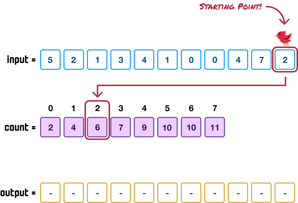
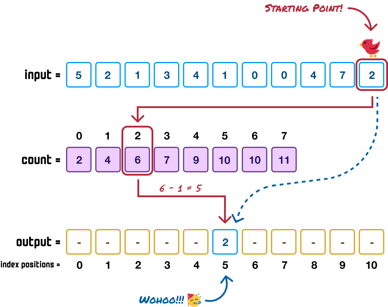
The value at the position indicated by the 2 value is 6. This 6 defines the position our last item in the input array (the one with the 2 value) will be when sorted. Because the 6 position needs to account for 0-based indexing, we reduce it by one and to find the index position 5 in our output array:

Now that we have found the sorted position our 2 value will be in, we can go ahead and place it in there:

There is one more step remaining. In our count array, we will decrement by 1 the stored value at index position 2 to indicate that we have already used it. In our case, the stored value of 6 will now become a 5:

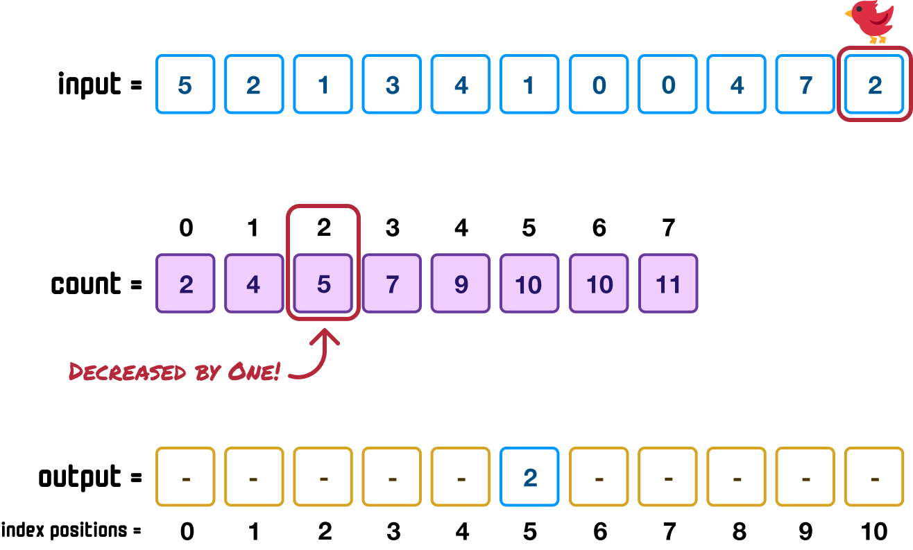
This is to ensure that any future attempts to find out where to place a value of 2 will not create a collision and overwrite a previously sorted value. When we encounter a 2 in our input array again, this time we will see that its sorted position is at 5, so we will place it at index position 4 instead. We’ll get to these shortly when we encounter our two adjacent 0 values in the input array, so don't worry too much about this detail just yet.

Ok, phew! What we saw was a very slow and detailed look at how we figure out how to place an unsorted item in the correct sorted position. We are going to speed things up a bit and repeat these similar steps. Next, we go down our input array to the next item, which has a value of 7. We know that 7 has a count value of 11, and this means its index position in our output array will be one less than that, which is 10:

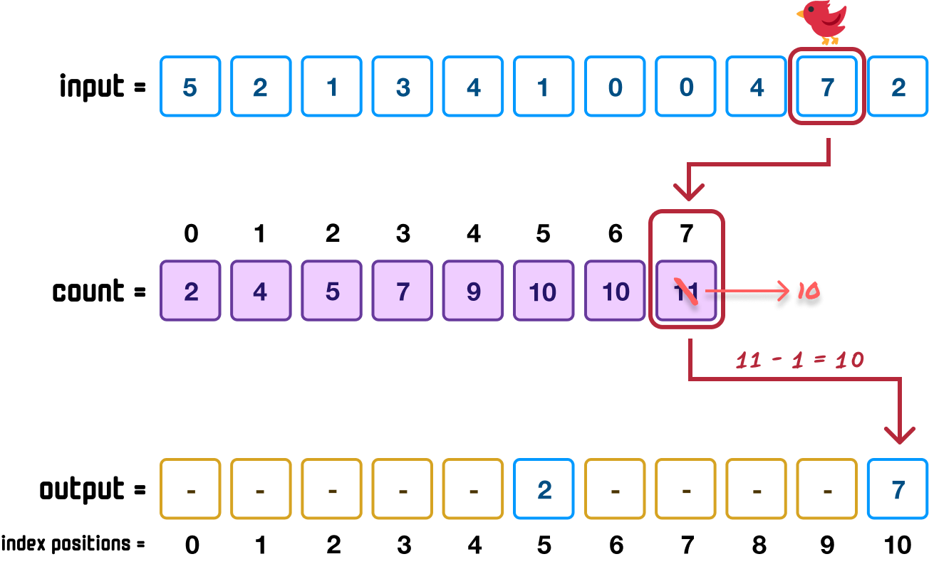
We also decrement the value of 11 in our count array to 10 to account for any future instances of 7 (if any!) finding a new location.

Going down our input, our next value is 4:

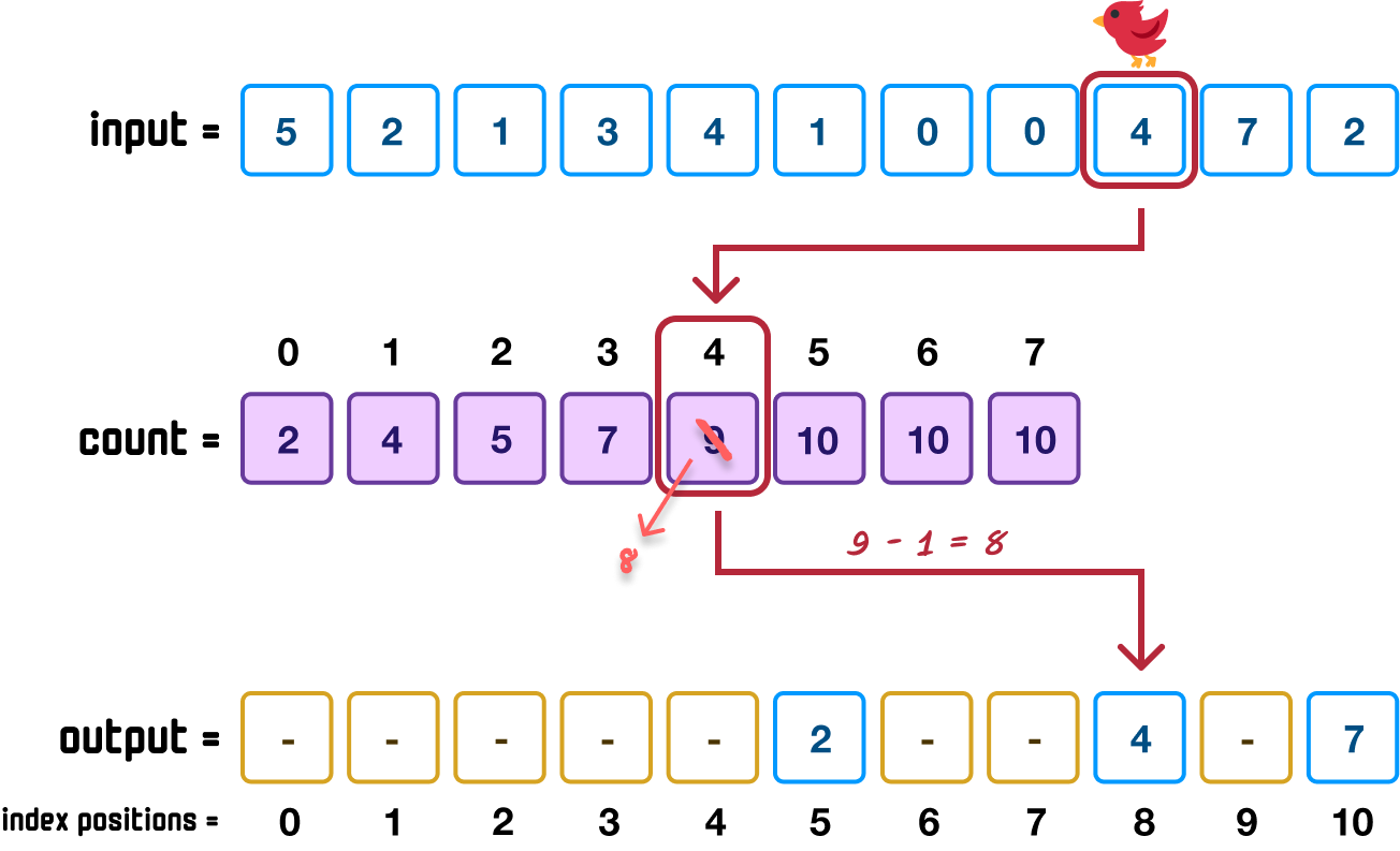
This 4 value maps to position 9 in our count array, and this means that 4 goes into index position 8 (9 minus 1) in our output array. As our last sub-step, we decrement the value of 9 to 8 in our count array.

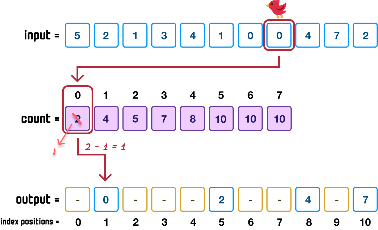
Next up we have a 0 value, and the steps we saw earlier repeat:

Moving along, we have another 0 value. When we repeat the steps, the state of our three arrays will be as follows:

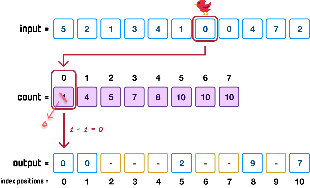
Because this is the second time the 0 value is being placed, we can see the importance of decrementing the position value in our count array after placing our item. When we encountered 0 for the first time a few steps ago, the corresponding count value was 2. After placing that first 0, we decremented the count value to 1. This ensured when we encountered 0 again in this step, because the corresponding position was now 1, we were able to place it at index position 0 in our output array and not have to deal with a collision.

At this point, you should have a good understanding of how each subsequent item from our input array will go through the count array and then be properly placed in the output array. At the end of all of these steps, the final state of our three arrays will be as follows:

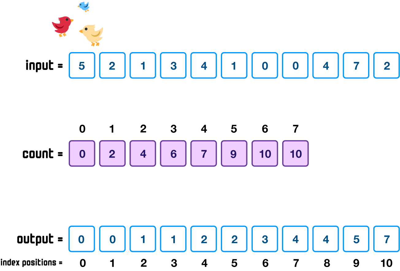
Of course, the only detail we really care about is what the output array shows, and what we see there is a properly sorted array.

Counting Sort Implementation

Now that we’ve seen how counting sort works using words and pictures, let’s go one level deeper and look at a JavaScript implementation of counting sort:

function countingSort(input) {
  // Find the maximum element in the array
  const max = Math.max(...input);

  // Create a count array to store the frequency of each element
  const count = new Array(max + 1).fill(0);

  // Count the occurrences of each element
  for (const num of input) {
    count[num]++;
  }

  // Calculate prefix sum to store the position of each element in the sorted array
  for (let i = 1; i <= max; i++) {
    count[i] += count[i - 1];
  }

  // Create an output array to store the sorted elements
  const output = new Array(input.length);

  // Place elements in the output array based on counts
  for (let i = input.length - 1; i >= 0; i--) {
    output[count[input[i]] - 1] = input[i];
    count[input[i]]--;
  }

  // Return the sorted array
  return output;
}

// Example!
let unsortedArray = [5, 2, 1, 3, 4, 1, 0, 0, 4, 7, 2];
let sortedArray = countingSort(unsortedArray);

console.log(sortedArray); // 0, 0, 1, 1, 2, 2, 3, 4, 4, 5, 7

Take a moment to walk through what this code is doing. There are a few things to notice here:

1. Notice how all of the code maps neatly to the various counting sort steps we looked at earlier.
2. We are doing no comparisons between values at any point here! This further underlines the point that counting sort is not a comparative sort at all.

The trickiest part of the counting sort implementation is making sense of the various array-related accesses we are doing. We have our input array, count array, and the output array. We take numbers from one, add it to the other, do some more adding, and then place a value into the correct location in the end. Compared to iterative functions or recursive calls that we’ve seen with our comparison-based sorting algorithms, I’ll take a bunch of loops and array accesses any day of the week. Maybe that is just me! 😅

// Place elements in the output array based on counts
for (let i = input.length - 1; i >= 0; i--) {
  output[count[input[i]] - 1] = input[i];
  count[input[i]]--;
}

Performance Characteristics

We started off by saying that counting sort runs in linear or O(n) time...under certain conditions. The following table is a quick summary of the best-case, average-case, and worst-case scenarios:

This looks very nice, but there is something subtle here that glosses over a lot of variation. As you can guess, by saying under certain conditions to qualify the linear-ness of counting sort, you know there is a catch. The catch is that the range of values we are sorting needs to be around the same size as the total number of values in our input.

Diving into Time Complexity

Taking our example from earlier, the largest number in our input was 7:

This means the range of numbers our sort will need to deal with goes from 0 to 7 for a total of 8 values. A good proxy for this is the size of count array, for we know its size will mimic the range of numbers from input as well. We will get more precise and give a label to both our input size and the range of numbers. Our input size will be designated as n, and the range of numbers in our input will be designated as k:

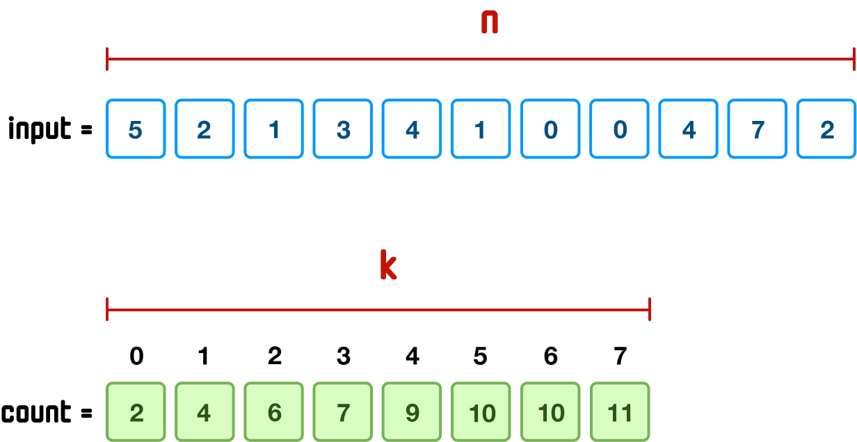
When we tie this with how counting sort works, we know that we loop through our input and count arrays a few times to calculate the final position of each unsorted item in our output array. Running a loop only a few times is not a major problem, so we can approximate counting sort's running time by saying O(n + k). This results in a linear running time only if n and k are similar.

If the range of k is very large, for example, it is on the order of n², then O(n + k) is no longer linear. It will be the max of whatever value is the largest, and it would be that the running time is O(n²) because k is n². We can see this play out in the following example:

The value of n here would be 7 because we are trying to sort 7 values. What would the value for k be? Because k corresponds to the range of numbers in our input, it would be the maximum value...which is 1,390,502! The implications of this can be seen in our count array:

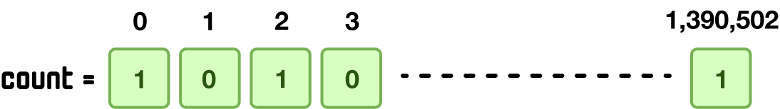
Our count array will have 1,390,503 entries whose index positions go from 0 to 1,390,502. No matter how we look at it, that is a massive array for just 7 numbers.

This isn’t very efficient both from the time it will take to iterate through all of the items as well as the amount of memory we need relative to the size of the initial data we are trying to sort. With n being 7 and k being 1,390,502, k is something around n⁷. This would mean that O(n + k) would be O(n⁷). That’s not very fast at all. It is far slower than some of our worst performing comparison-based sorting algorithms.

Tying this all together, the relationship between n (size of the input) and k (range of numbers in the input) is what determines whether counting sort runs in linear time or not. For this reason, counting sort works best when the range of numbers we are dealing with is limited and within a narrow range. This is a detail that we'll always see called out to clarify why counting sort isn't always the fastest algorithm nor the default choice for all sorting situations.

Understanding the Space Complexity

Similar to the performance, the space complexity for counting sort is also O(n + k). Counting sort requires additional space proportional to the size of the input array (n) plus the range of the input values (k). For large ranges, such as the example we saw a few moments ago, the additional memory required to deal with the count array could become very impractical.

Speaking of space, because of how counting sort is implemented, it isn’t considered an in-place sorting algorithm. It requires additional space proportional to the range of input values (k) for storing intermediate counts. In-place sorting algorithms modify the input array without requiring additional space, which is optimal from a memory usage point of view.

Conclusion

Counting sort has a lot of things going for it, but it also has some issues that we need to keep in mind. In terms of what it is great at:

• Really really fast: Counting sort operates in linear time O(n+k), where n is the number of elements and k is the range of the input values, making it highly efficient for datasets with a limited range.
• Stability FTW: Counting sort preserves the relative order of equal elements, ensuring stability in sorting, which is essential in various applications.
• Simple implementation: Counting sort has a straightforward implementation made up of loops and arrays, making it easy to understand and implement, even for those new to sorting algorithms.

In terms of what makes counting sort a bit meh:

• Limited applicability: Unless we do a lot of special work, counting sort is restricted to sorting arrays of non-negative integers, limiting its use in scenarios involving other data types or negative numbers. For sorting arbitrary types of data "out of the box", a comparative sorting algorithm would be your best bet.
• Space complexity: Counting sort requires additional space proportional to the range of input values, which can be a drawback when dealing with large ranges in memory-constrained environments. This is especially true if the range of input values is significantly larger than the number of elements (k >> n), counting sort's space requirements may become impractical, leading to...inefficiency! 💀

Not all non-comparative sorting algorithms exhibit some of these same problems. There are better implementations. In the future, we'll look at one such improved implementation, the Radix Sort.

Just a final word before we wrap up. If you have a question and/or want to be part of a friendly, collaborative community of over 220k other developers like yourself, post on the forums for a quick response!