The Merkle tree, also known as a Hash tree is named after mathematician and computer scientist Ralph Merkle (and not the former German Chancellor Angela Merkel or Markl from Howl’s Moving Castle):

Merkle trees are good at identifying whether some data in a dataset has changed. This seemingly simple capability makes them extremely popular across a variety of everyday situations. Merkle trees play a big role in ensuring messaging apps, software updates, cloud storage services, Git version control systems, file sharing solutions, blockchains, and a whole lot more work well.

In the following sections, we’ll dive into what Merkle trees are, how they work, and why they are just so popular across so many of the things we do in our digital world.

Onwards!

What is a Merkle Tree?

To better understand what Merkle trees are and how they work, let’s start by looking at an example. Imagine we are building a cloud file backup service similar to popular ones like Dropbox or Google Drive. We’ll call our service DriveBox:

DriveBox’s goal is to ensure that files stored locally are backed-up to a cloud server, and any changes to the local files are reflected in the cloud version as well.

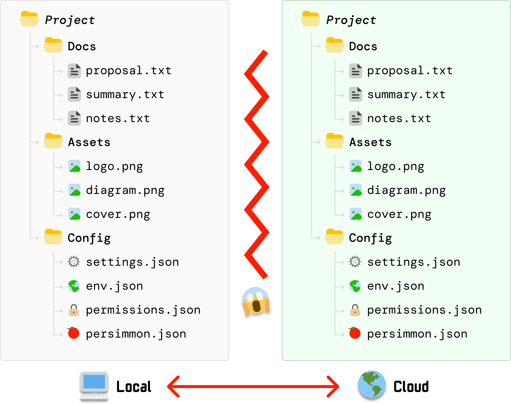
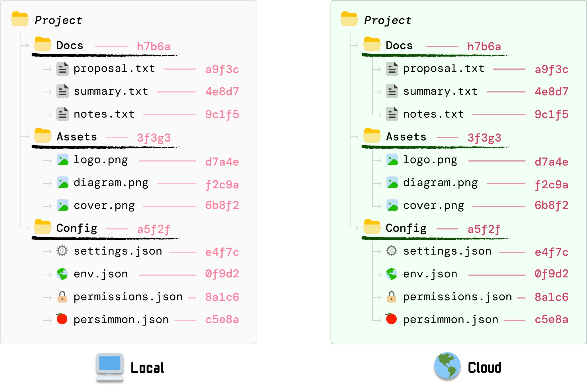
Let’s say the files we have in our local machine look as follows:

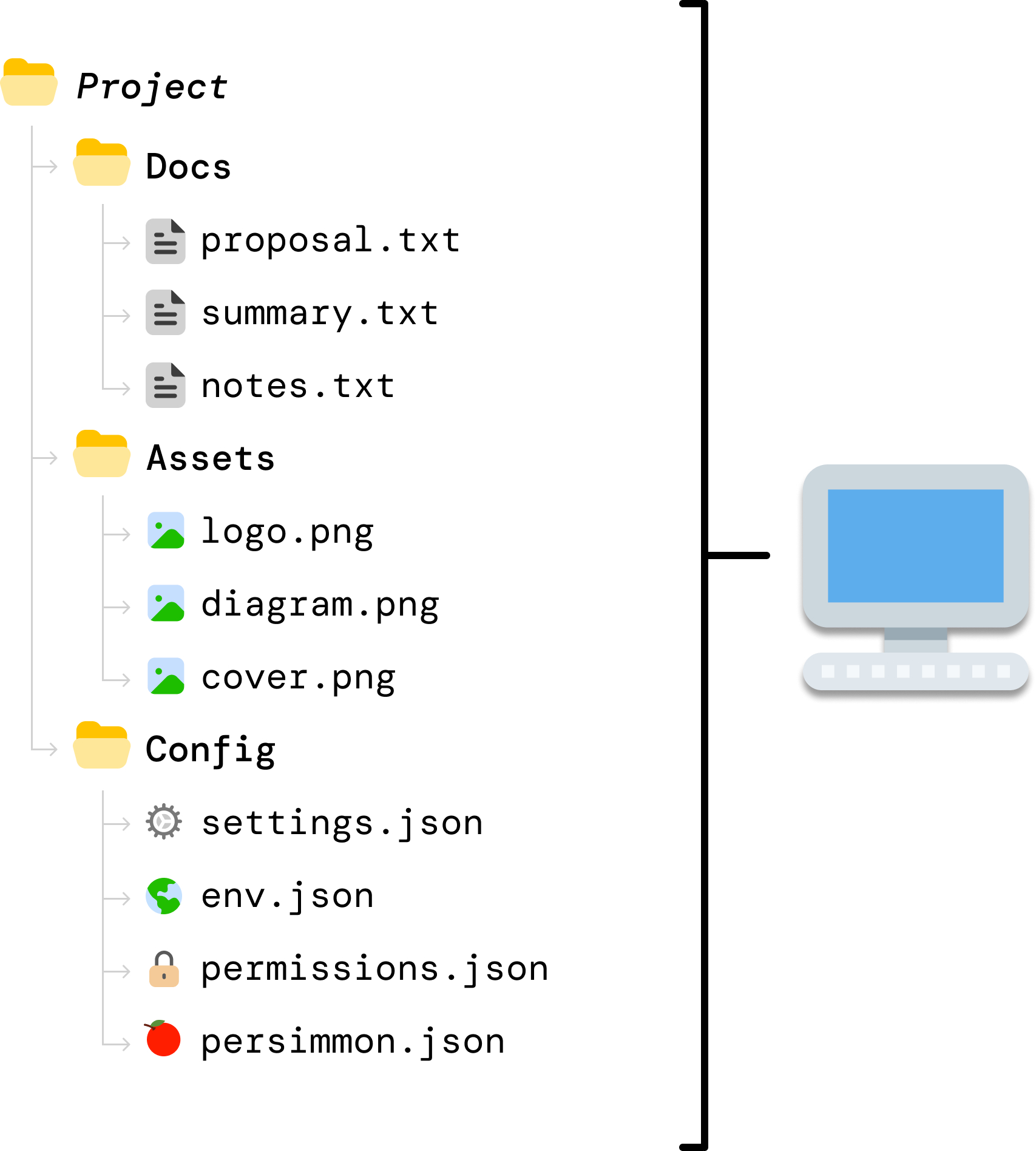
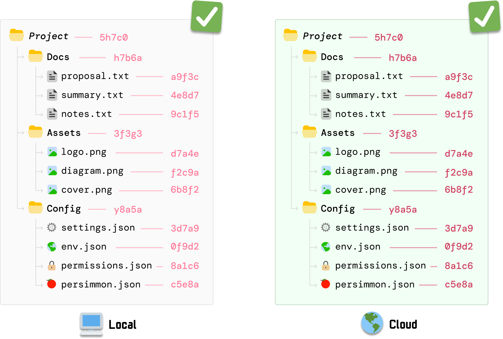
DriveBox has created a backup of these files on the cloud server. When we look at the cloud server contents, we can see that these files are also already perfectly synced there as well:

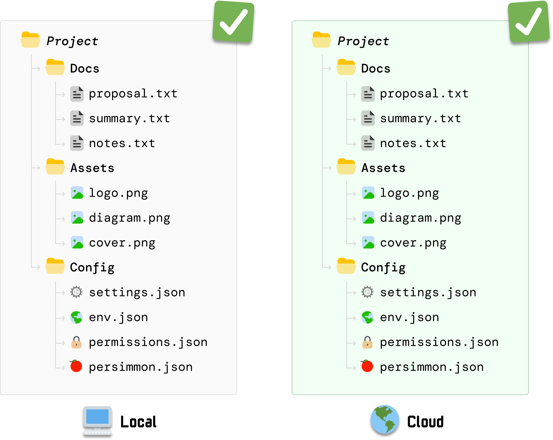
Take a mental snapshot of this moment where our local state and cloud state are identical. This is going to be the starting point for the exciting part of our example.

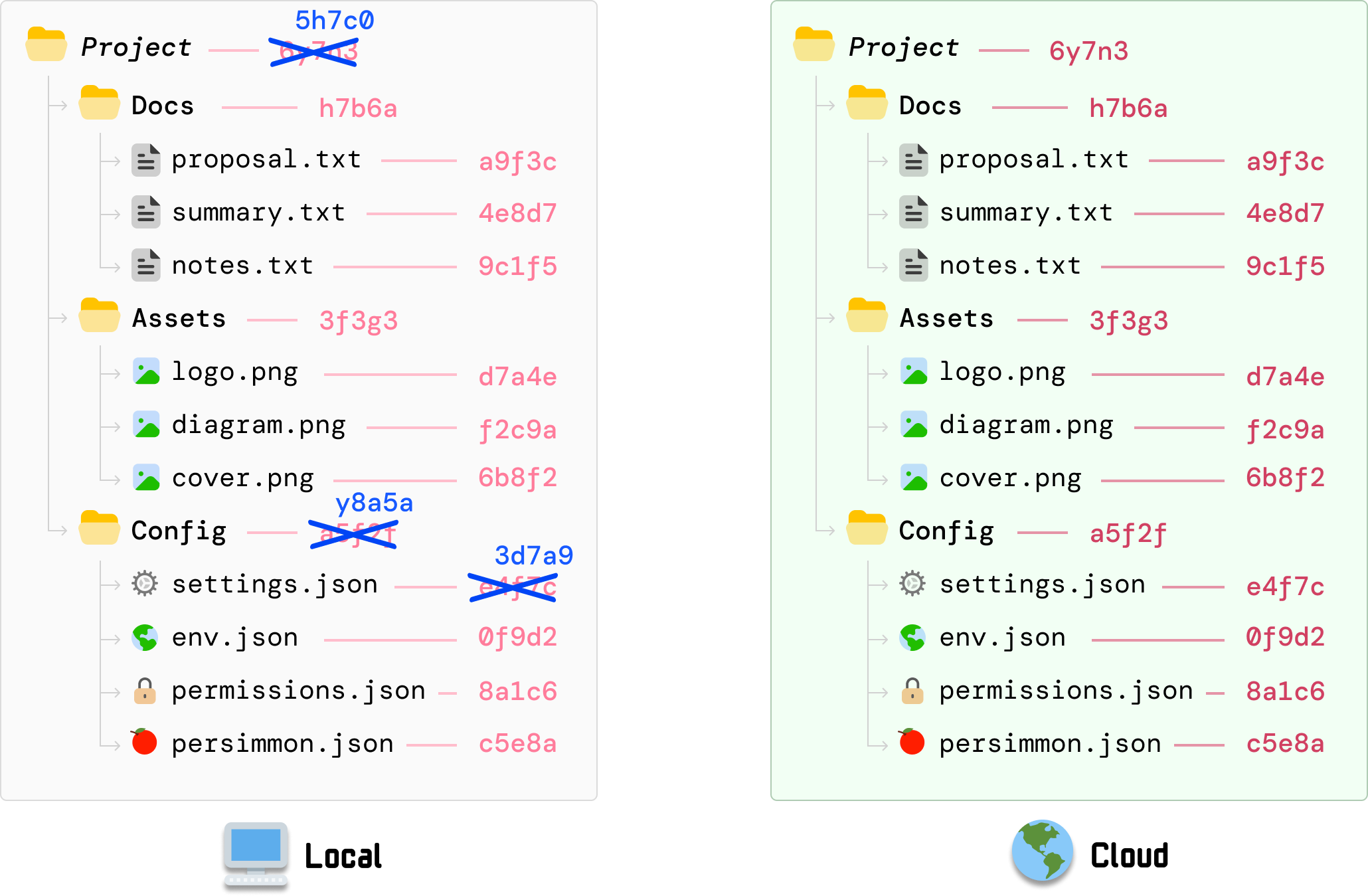
From this happy state where everything is in sync, we are going to make a change to one of our local files. We are going to make a change to settings.json. After we make the change and save it, we have a more recent change in our local settings.json file than its equivalent stored in the cloud:

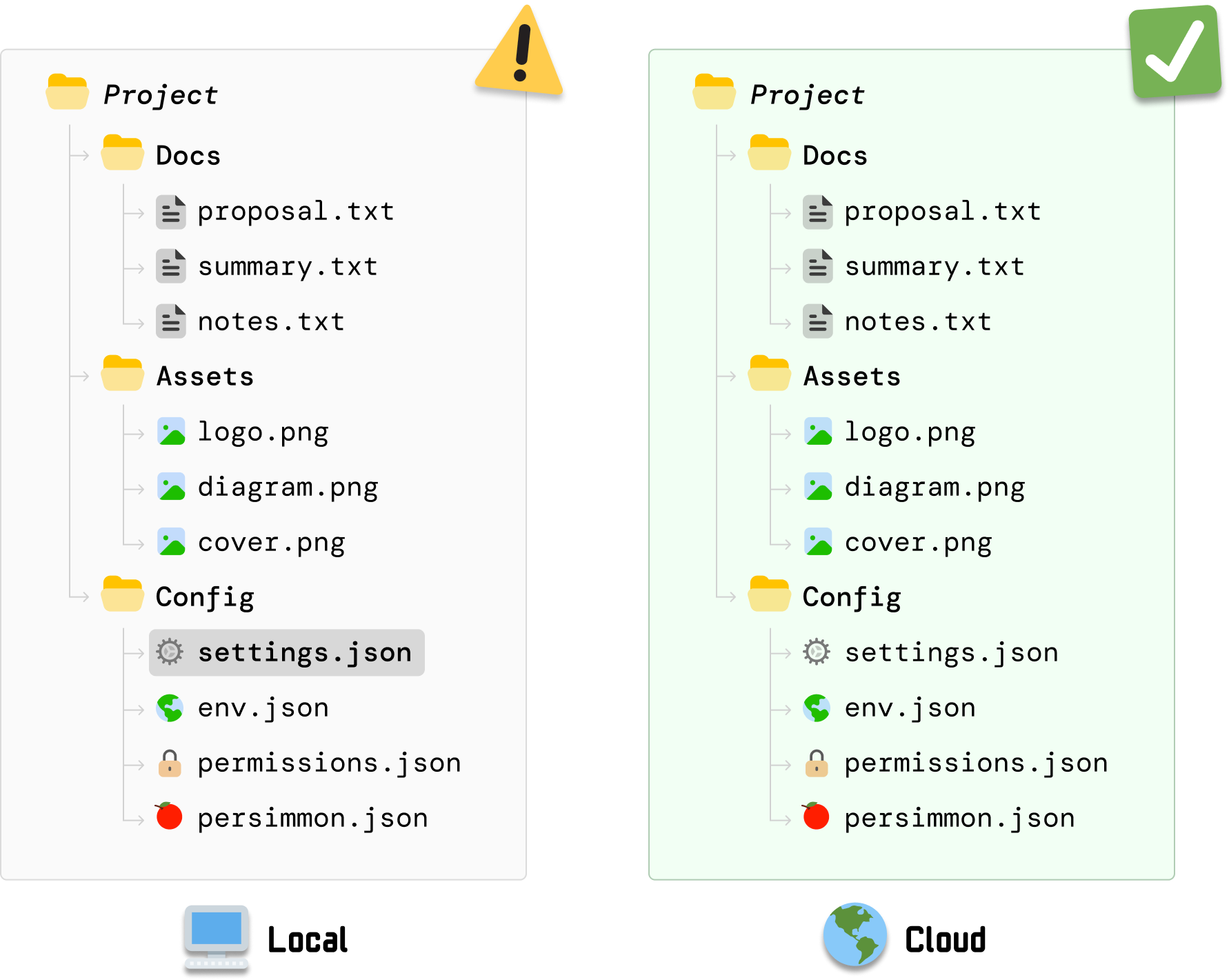
The local and cloud versions of our files are no longer in sync. Now, our desired behavior would be for DriveBox to detect this change to settings.json and update the cloud version to match what is available in our local machine. How DriveBox pulls off this behavior is where Merkle trees come in.

In a land far far away...

To highlight how Merkle trees can help ensure our updated settings.json file is synced across our local machine and cloud server, we are going to take a step back and look at what approaches we can use in a world where Merkle trees haven’t been invented yet. This is a good exercise in helping us think through the full complexity of this problem.

Take a few minutes and brainstorm some possible approaches you can take. Keep in mind that whatever solution you come up with needs to:

1. Work for a large amount of files
2. Accurately identify changed files
3. Work across multiple devices
4. Reduce unnecessary wasted work

After you’ve thought through some approaches, let’s look at three possible solutions.

Approach 1: Re-upload the entire folder with each file change

This is the ultimate boil the ocean approach where we trigger a full re-upload of the Project folder whenever any file on our local machine changes:

Even unchanged files will get uploaded to avoid any discrepancies. If we take a step back, this approach certainly gets the job done, but it isn’t great because it:

• Wastes bandwidth and battery
• Is slow on large folders or slow networks
• Scales terribly as folders grow. Imagine uploading thousands and thousands of files each time a single file is updated.

This solution is quite inefficient. Ideally, we will want to only upload our changed files (like settings.json) and leave unchanged files alone.

Approach 2: Compare file lists and timestamps

This approach uses known markers for when something was (potentially) last updated. The markers we will use are the timestamp and the listing of files:

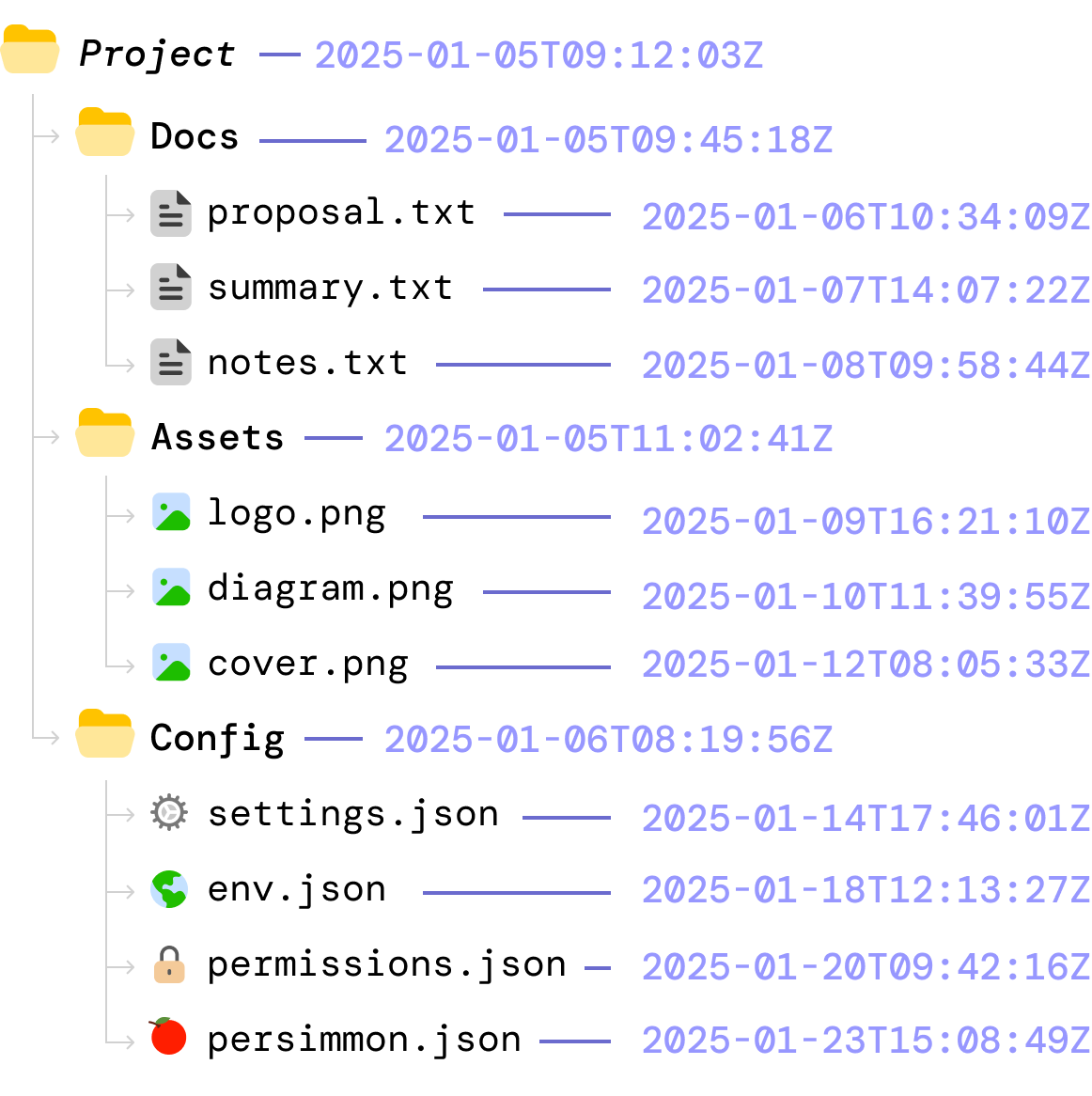
In this world, what happens is the following:

• Our local machine sends file names and the current timestamps to our cloud server
• Our cloud server compares the local version of file names and timestamps to its own version of file names and timestamps.
• When our cloud server compares timestamps, it will detect that settings.json is more recent than what it has stored currently
• This discrepancy is fixed by ensuring the local copy of settings.json is sent along to replace the older copy in our cloud server

This approach seems to work well, but relying on timestamps and file lists is error prone. Some of the issues we will run into are that:

• Clocks drift across devices where the time on your local device won’t be in-sync with the cloud. This could lead to constant uploads of every file because the time drift will make every file seem like it has been updated.
• Copying or restoring files usually preserves timestamps, which hides the fact that a change could have been made
• Malicious or buggy clients can lie. While this may not apply to DriveBox, it is worth keeping in mind when looking at this solution broadly!
• There is no guarantee file contents actually changed despite timestamp updates, so there may be wasted uploads. Back in the day, antivirus tools were notorious for changing timestamps when they simply scanned a file.

The challenge is that timestamps and file lists only describe when files were touched and how folders are structured. They don’t specify what the files actually contain. Because this metadata can be inaccurate, inconsistent, or misleading across devices, we need to think of better approaches.

Approach 3: Hash every file on every sync

One thing we know is that hashing is a fast operation, and the hash value for a file can be made dependent on the file contents. Knowing that, we generate a hash value for each file both locally and on the cloud:

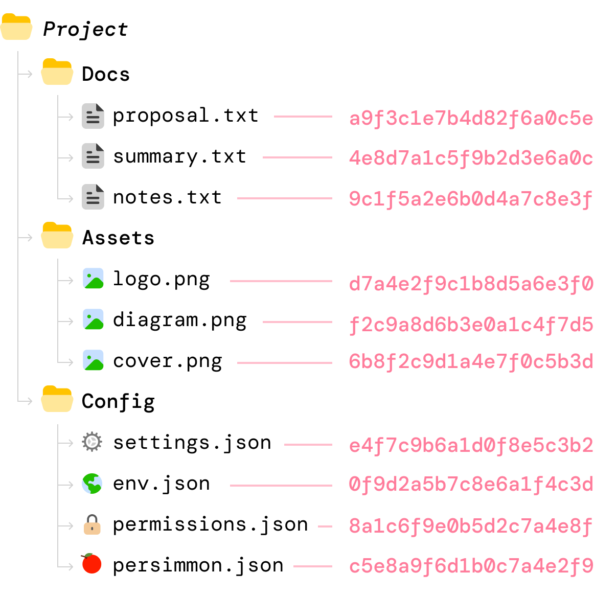
When a file’s content changes locally, we compute the new hash value for that file:

Because we have the hash value for each file on the server, the syncing between our local machine and the cloud server can first involve only comparing hash values. Whenever the hash values don’t match, it is safe to say that the file’s contents have been changed. When that happens, we can upload only those files whose hash values don’t match.

This approach seems like a winner, right? Hashing is a fast operation. We have an airtight way of detecting the files that have changed. Well...the issue here is subtle but just as problematic as our discarded earlier approaches.

Here we assume the client always detects every file change and that its record of the server’s last-known hashes is never stale. The problem is that filesystem notifications can be missed and/or other devices can update the same files while this client is offline. When either happens, the client has no reliable way to know that its view of the folder is incomplete, which can lead to inconsistencies or force expensive full rescans to recover. We shouldn’t discard everything about this approach, though. There are some good ideas here that we will want to keep.

Merkle Trees to the Rescue

We looked at three approaches for how we can ensure files stay in-sync between our local client and our cloud server. Some approaches worked better than others, but they all had some serious gaps. This is where Merkle trees come in. They bring some interesting design choices that allow us to solve our file synchronization problem without also bringing along some of the unwanted side effects.

The best way to understand these design choices is to use a Merkle tree to continue working through the same example we have been looking at so far.

Starting Point

Reliving a moment from a few paragraphs ago, our starting point is where we have our local files and our cloud files in-sync:

At this moment, there are no file changes. Everything is the same across our local and cloud server versions.

Step 1: Hash each leaf node (file)

During the initial sync, each file’s contents are hashed to produce a unique fingerprint, and this happens both locally and on the server:

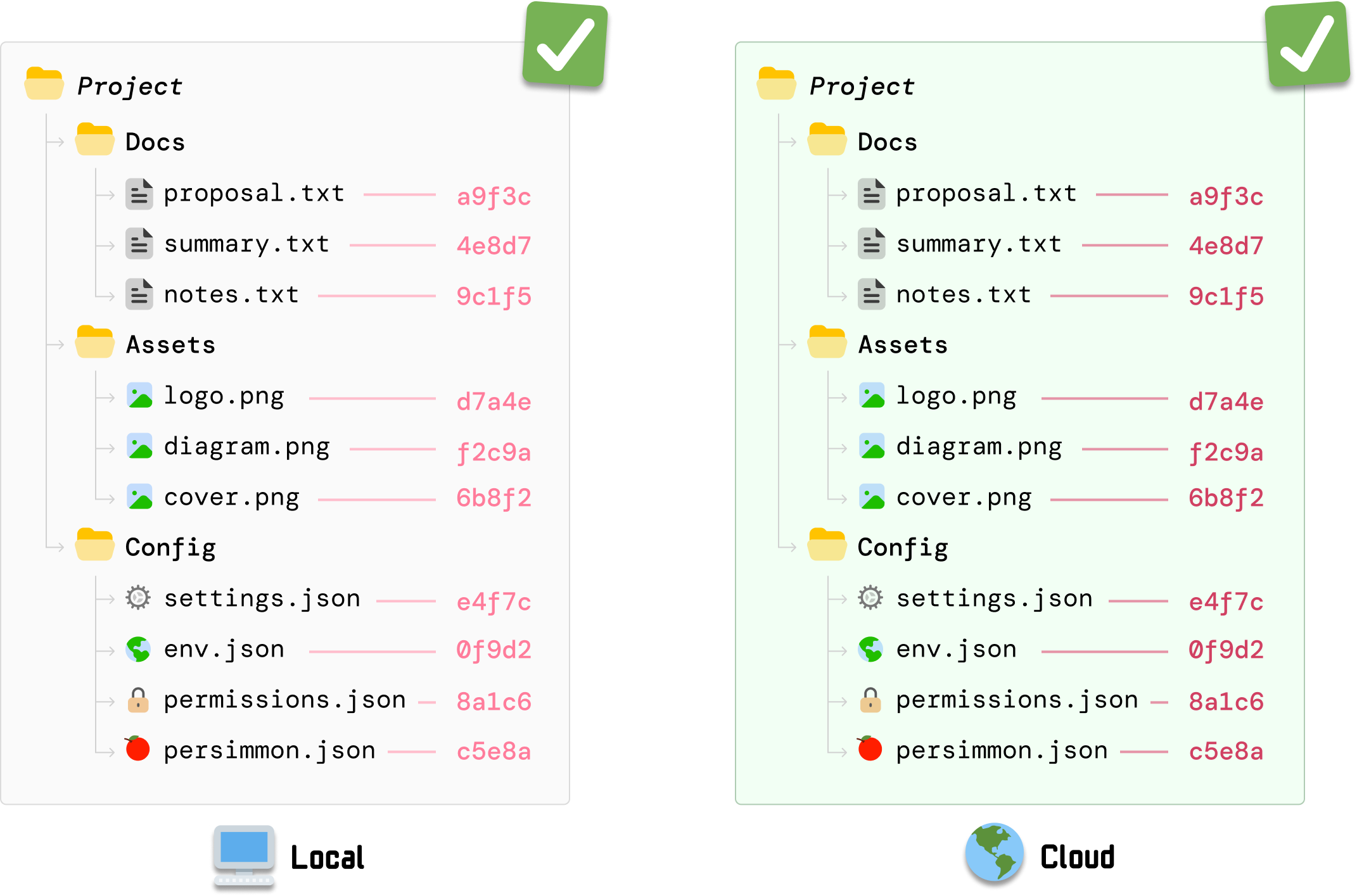
The detail to note is that the same hashing function is used by DriveBox both locally as well as on the server. This ensures that, for the same file, the same hash value is generated.

Step 2: Build Merkle hashes for each folder

What we’ve hashed so far are just the individual files. Next, we need to hash the folders. The way we do this is by hashing the hash values we generated for each file under each folder:

DocsHash    = Hash(proposal || summmary || notes)
AssetsHash  = Hash(logo || diagram || cover)
ConfigHash  = Hash(settings || env || permissions || persimmon)

If we had to visualize this, we can now see our folder hashes as follows:

There are a few things to note here:

1. The order in which we hash each file is important. We hash them in what is known as a stable order. “Stable order” means that the child hashes are always combined in the same deterministic sequence, regardless of machine, operating system, or timing. This means the same folder contents always produce the same folder hash. In our example, we hash them in a top-down order.
2. To emphasize an important detail, we hash only the hash values of each file in each folder. We don’t hash the file contents again. That would be unnecessary work.

At the end of this step, each folder under Project now has a folder hash that represents every file inside each folder.

Step 3: Build the root hash for the entire project

Now that we have the hash values for each file and their parent folders, the last step is to generate a hash value for the root. We do this by taking each subfolder’s hash values and hashing them:

ProjectHash = Hash(Docs || Assets || Config)

Visualized, this looks as follows:

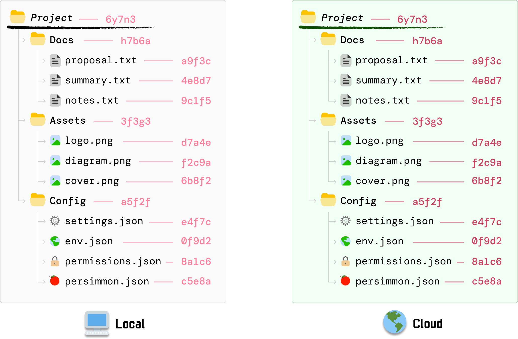
Just like earlier, the hashing order is stable. We hash the subfolder hash values in top-down order, and the values are still identical between our local copy and the cloud copy.

Also, all this talk about hashing made me think of...

Step 4: We change settings.json

Now, things are going to get interesting. We edit our local copy of settings.json where the file contents have now changed. Whenever a file changes, what we do next is recalculate the hash value for this file:

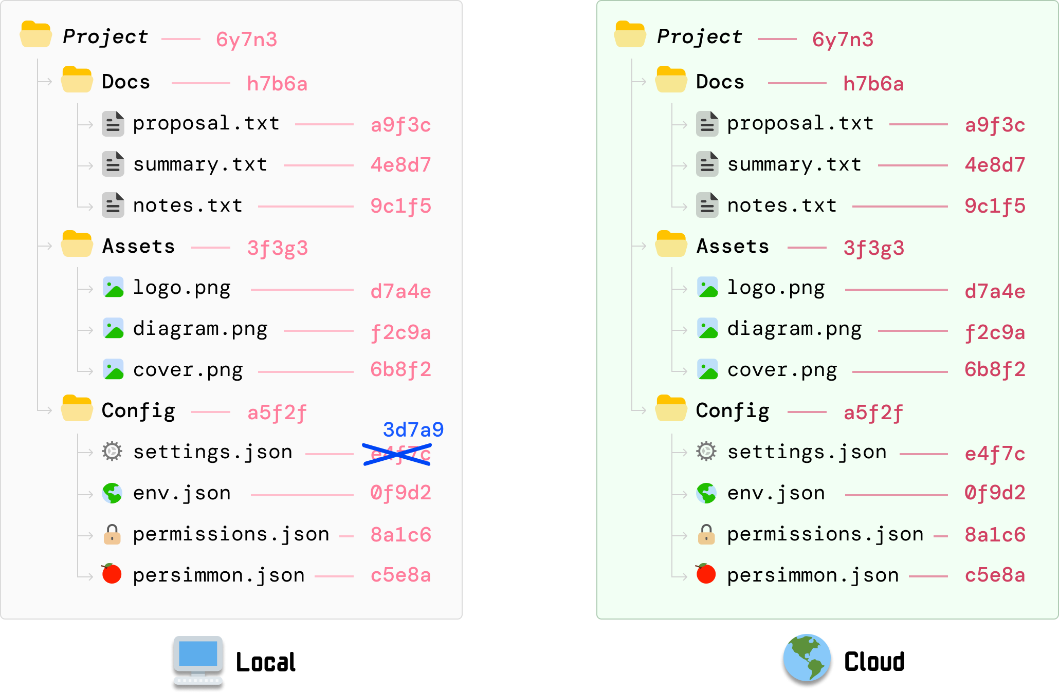
The old hash value (34f7c) is now replaced with the new hash value (3d7a9). All other file and folder hashes remain unchanged...for now. Our cloud copy of the files also remain unchanged, for our cloud version has no knowledge of what has just happened on our local machine.

Step 5: Hash changes propagate upward to the root

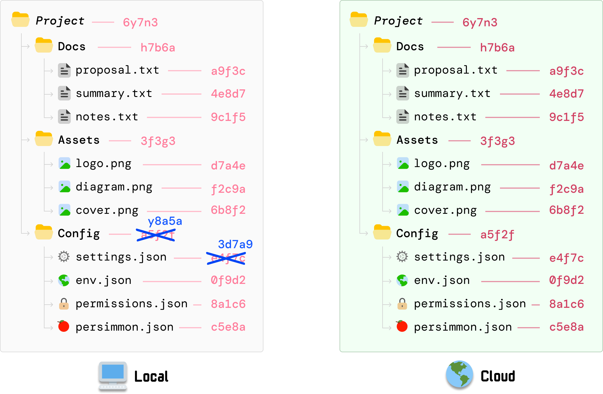
Because the hash value for the Config folder depends on settings.json, its value is now stale. It needs to recalculate the hash value to reflect the new settings.json contents, and we can reuse the individual hash values for the files that have not changed:

We don’t just stop here. Do you know why? The hash value for our root Project folder is based on the earlier calculated hash value for Config. It now needs to change:

This value gets calculated by taking the individual hash values for our three subfolders and updating to the new value in the same top-down order. This is a recursive operation that will keep continuing until we reach our root folder, but in our example, our root folder is Project and we have nowhere further up to go.

At this moment, the part to highlight is that our change to settings.json resulted in the following hash values changing: settings.json, Config folder, and Project (aka root). The hash values for the other files and and folders don’t change.

Step 6: Detecting the change on the server

From our local settings.json modification, we know our root hash value has changed as a result. At this point, the root hash value locally is different than what is stored on our cloud server:

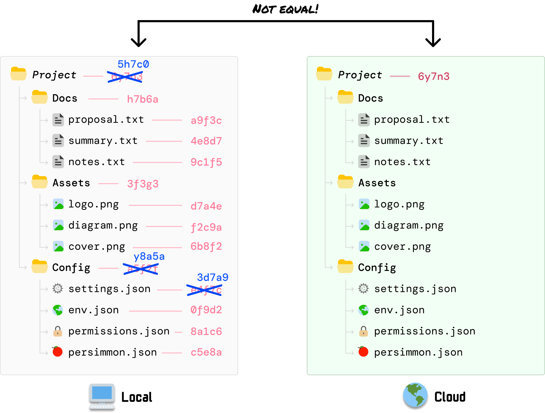
This one single check indicates that something has been updated in the files we are syncing. What our cloud server doesn’t know is exactly what has changed. It only knows about the root hash having changed, and that detail is enough for it to start investigating further.

Step 7: Pinpointing the exact change (tree walk)

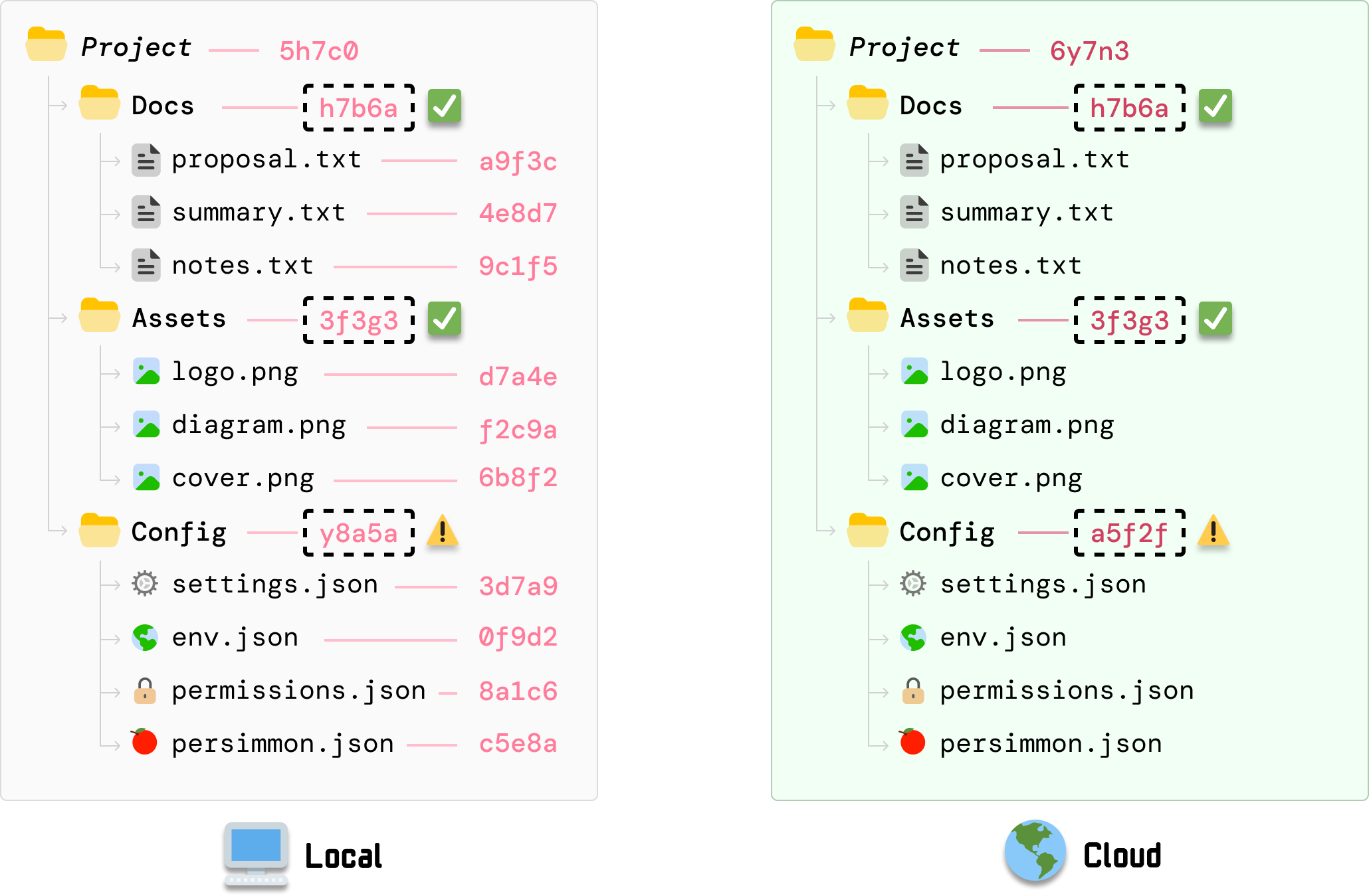
To identify what has changed, our cloud server will narrow the difference by comparing hashes level by level and communicating with the local client on what may have changed.

As it walks down the tree and looks at the Docs, Assets, and Config folder, it can compare the local client’s folder-level hash values with what the server had calculated earlier and identify that the hash value for Config is different:

Next, because the Config folder indicates a change, we continue the same approach and explore the Config folder further. When we compare the hash values for each file under Config, we can see that the value for settings.json has a mismatch:

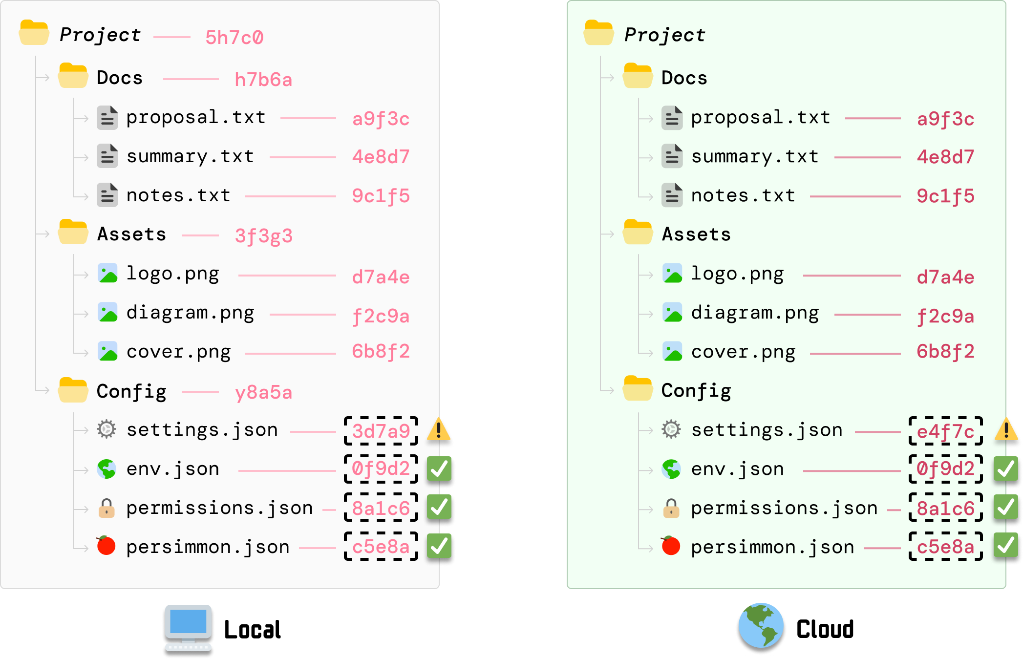
This means that DriveBox on our cloud server knows that our settings.json file has been updated. Because there are no child folders to explore further, we are at a leaf node and can safely say that the source of all of the mismatches is an outdated settings.json file.

Step 9: Synchronizing the change

At this step, our cloud server sends a request to our local client to send the new settings.json file. Once settings.json has been sent and the old settings.json file overwritten with the new contents, our cloud server will recalculate the hash values for:

• The updated settings.json file
• Config folder
• Project (root) folder

Note that any change to the hash values will require navigating back up the tree and ensuring the hash values for every parent folder are updated. At the end of these recalculations, the root hash value between our local client and our cloud server will now be identical:

Because our root hash value is built-up of all the hash values below it, identical root hash values indicate that we are now back in a state where all of our files are perfectly synced between our local version and the cloud version.

Performance Characteristics

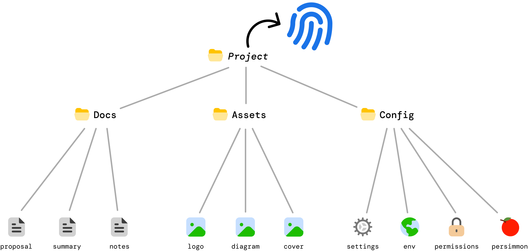
So what just happened? Think of a Merkle tree as a way for DriveBox to give our entire Project folder a single, trustworthy fingerprint that is built from the contents of every file inside it:

When this fingerprint is the same across our local machine and the cloud server, it is safe to say that all of our files are in sync. If the fingerprint changes, then somewhere in our collection of sync’ed files, something has changed. This was the case with our changed settings.json file. This approach for quickly detecting a change has a more formal name, and that is the Merkle proof. This is a name you’ll see in many descriptions of Merkle trees in the real world. More on that in a bit...

Taking a few steps back, we’ve been talking about Merkle trees in the form of our files/folders example. A Merkle tree is a...tree, so we can provide an alternate representation that looks more like the tree data structures that are everywhere in the data structures world. If we convert our files/folders visualization to look more like a tree, we will see something that looks more like the following:

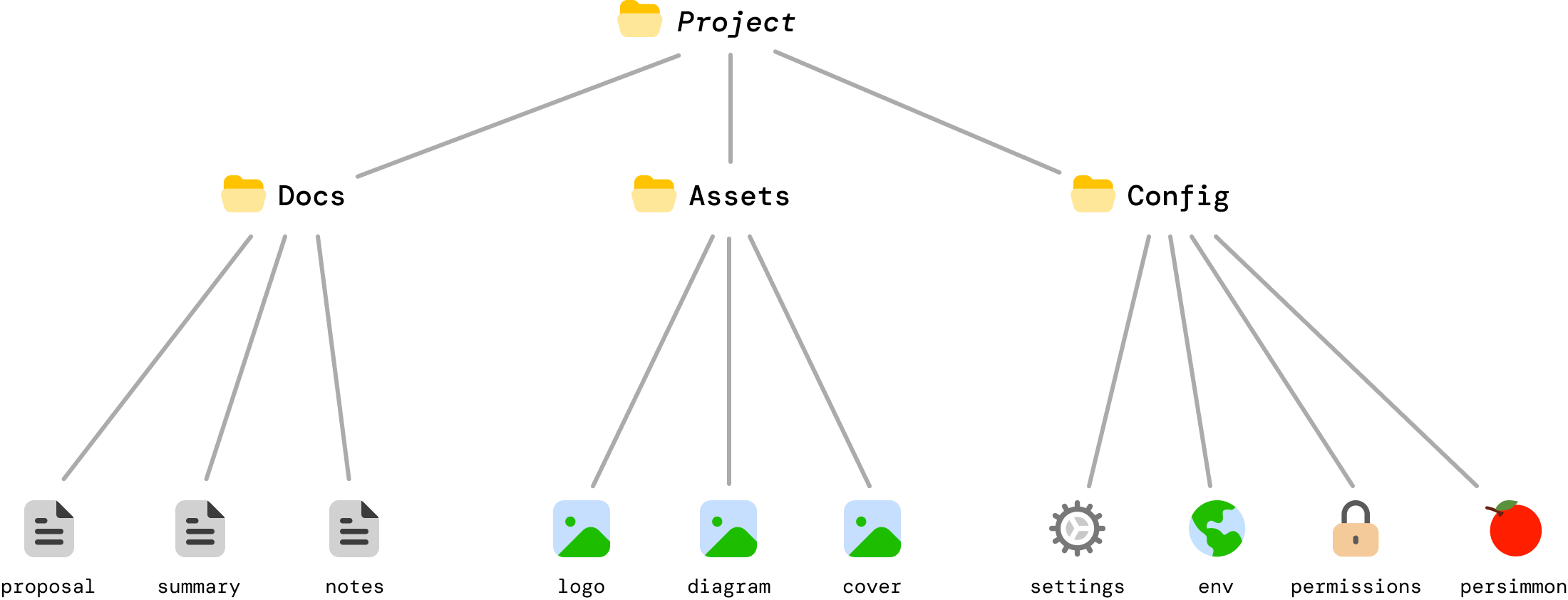
This is the same example as earlier. The only difference is in how it looks to us, but this visualization helps us better see how efficient a Merkle tree is. When a change is made to settings.json, the only bits that are impacted are settings.json itself and the Config and Project folders which rely on the hash value of settings.json for their own respective hash values:

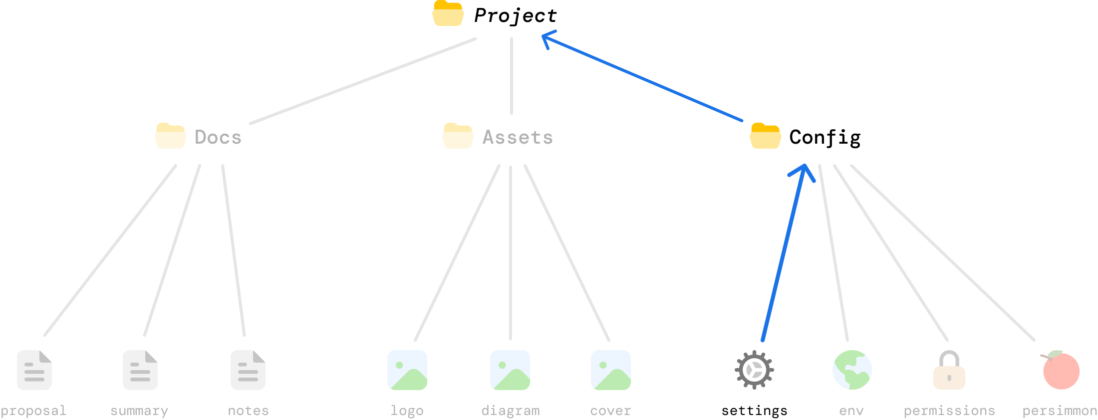
This makes Merkle trees very efficient! For a tree with n leaves, a Merkle proof only requires log_b(n) hashes where b is the branching factor, or number of children per parent. For a million files and we have a binary tree (branching factor of 2) structure, we’d only need about 20 hashes to prove that a file has changed. That’s pretty efficient!

Now, Merkle trees may have arbitrary children at each level. This is common when we are dealing with input data that isn’t neatly grouped or cleaned up to fit a binary (or related) tree format. When the number of children is truly arbitrary, kinda like our example where some children had three nodes and others had four, we can still say that the Merkle proof length is proportional to the tree height.

Height is logarithmic in n with base equal to the effective average branching factor (if the tree stays roughly balanced):

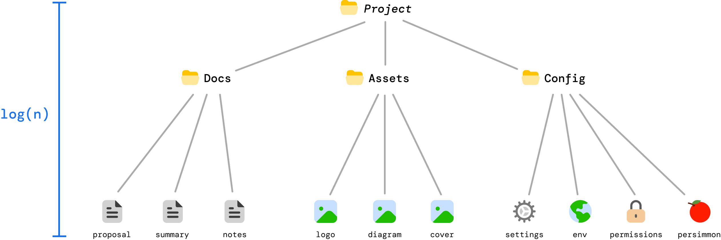
Worst case, our Merkle tree could be extremely unbalanced and resemble a linked list. In this scenario, the height is the same as the total number of items or O(n). Whatever advantages Merkle trees bring are completely lost, but Merkle trees used in practice are designed to avoid this degenerate situation by enforcing balance even if we have, to continue our files and folder example, a single folder with a million files in a flat list.

A Look at the Real-World Applications

We started off by saying that Merkle trees are used in many everyday scenarios. Now that we know more about how Merkle trees work, let’s take a slightly deeper look at how they are used in these everyday scenarios beyond the file syncing scenario we walked through.

Blockchain and cryptocurrencies

Bitcoin and other cryptocurrencies use Merkle trees to efficiently verify transactions. If we simplify what a block looks like, it will look as follows:

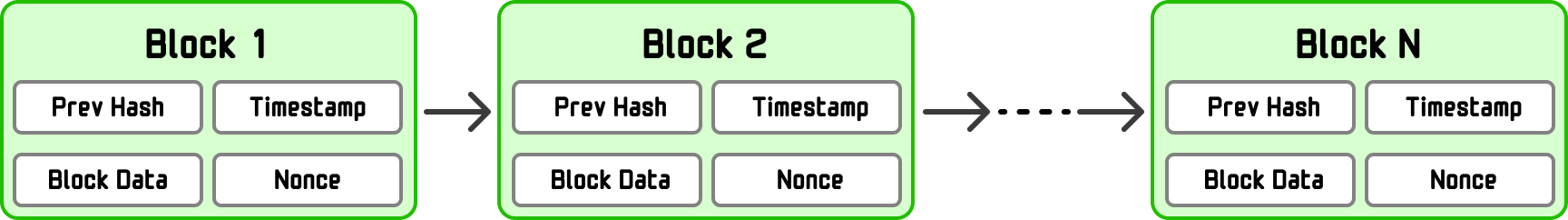
Not to get all blockchainy on you, but a block is usually split into two logical parts: (1) the block header and (2) the block data (aka body). What we see above is the block header. The block data is where we have our Merkle tree made up of all transactions in that block:

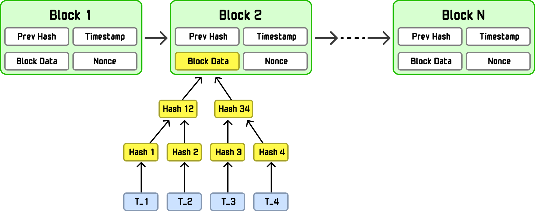
To be more specific, Merkle tree is built from the block’s transactions (T_1, T_2, T_3, T_4), which live in the block data. Once that tree is constructed, its Merkle root, a single hash that cryptographically represents all transactions, is written into the block header itself. This lets nodes verify that a transaction belongs to a block using a short Merkle proof, without downloading the entire block.

Git version control

Whenever we use a git-based solution like Github to keep our files in sync, Merkle trees are used behind the scenes. Have you ever seen these hash values as part of a commit?

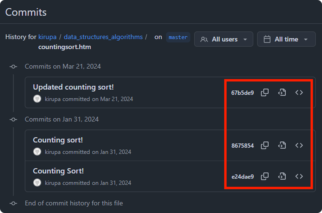
These hash values are there because git hashes every object (files, directories, and commits), and those hashes reference one another where file contents are hashed into blobs, directory listings hash those blob hashes into trees, and commits hash the root tree plus parent commit hashes and metadata. This is like a more souped version of the files/folders Merkle tree example we looked at where what gets hashed is more than just the file and folder contents.

Because each hash depends on the hashes beneath it, changing even one line of code changes the commit hash, and this is what allows Git to work the way it does in helping us keep files in sync. To go one level deeper, since commits can have multiple parents and share subtrees, Git is more precisely a Merkle DAG (Directed Acyclic Graph). In this graph variation, each node is identified by a cryptographic hash of its contents and the hashes of the nodes it points to, and the graph has no cycles (you can’t loop back to an earlier node). All of this is just a fancy of way of saying a commit hash cryptographically represents the entire repository state at that moment. If the hashes are out of sync, then something has changed and we need to re-sync to maintain consistency.

Distributed Databases

Systems like Apache Cassandra and Amazon DynamoDB replicate their data across multiple databases to ensure that a failure in a single database doesn’t bring everything down. To ensure the replicated copies are in-sync, these database use Merkle trees to maintain consistency and quickly catch inconsistencies:

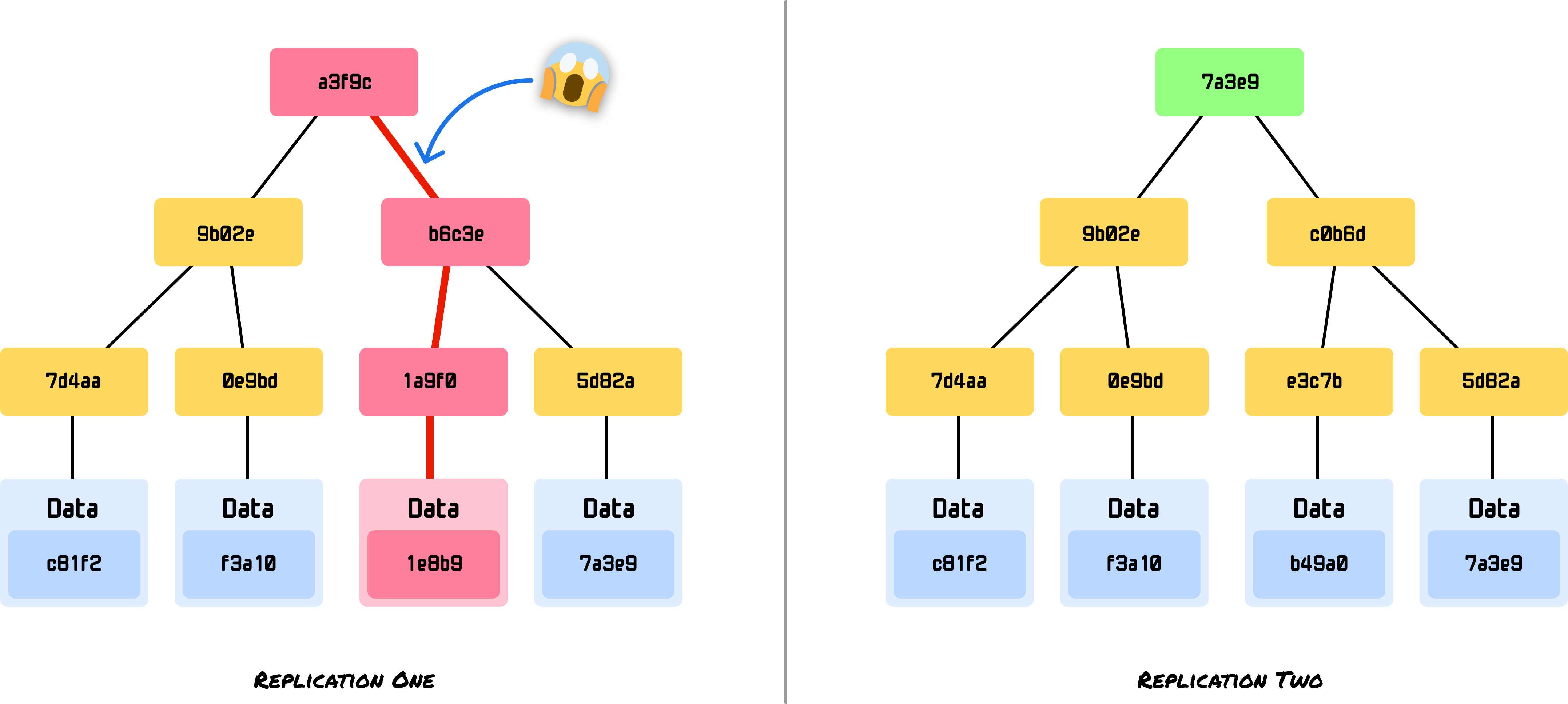
Instead of comparing potentially gigabytes of data, these kinds of systems can compare root hashes and then drill down to find discrepancies and sync only the files that have changed. In mission-critical workloads with many database transactions per second, this efficiency is important to avoid situations where data stays out of sync for long periods of time.

File Verification Systems

This scenario is nearly identical to the DriveBox example we saw earlier! An example of a distributed storage system that is one level deeper than applications like Box/DropBox/OneDrive/etc. is IPFS (InterPlanetary File System). IPFS uses Merkle trees to create something known as content-addressed storage, as seen in this visualization from their blog:

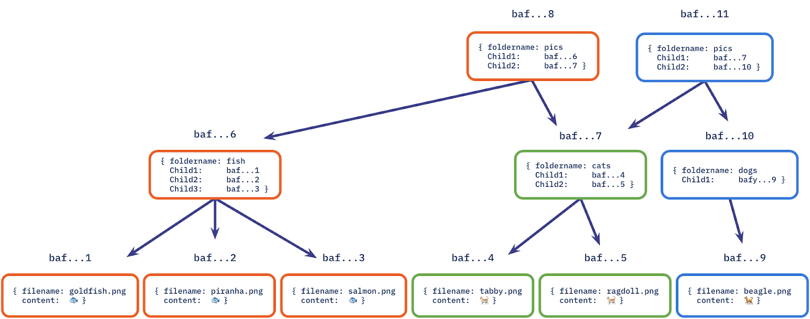
Files are broken into blocks, each block is hashed, and a Merkle tree is built. The root hash becomes the file’s unique identifier.

Certificate Transparency

When we visit a secure website (https://), our browser is shown a TLS certificate that claims, I am example.com, and a trusted Certificate Authority (CA) vouches for me.

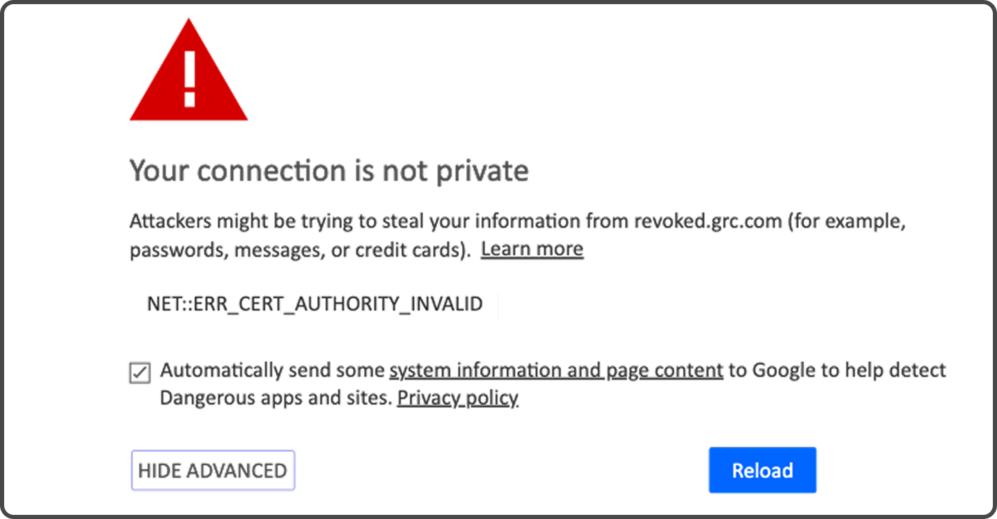
Historically, browsers mostly trusted that CAs did the right thing. The problem? Sometimes they didn’t. A CA could accidentally (or maliciously) issue a valid certificate for a domain to the wrong party. That creates a problem where attackers can impersonate real websites and users would never know, but our browsers typically sniff out these problems. You may have seen warnings like this in the past:

How do our browsers know that a site’s trustworthiness is a bit flaky? This is where Certificate Transparency (CT) comes in. The idea is simple but powerful: Every certificate issued by a CA should be publicly visible so that domain owners and browsers can audit what’s been issued.

So instead of certificates being quietly created behind closed doors, they’re appended to public, append-only logs. Anyone can inspect these logs and catch any issues.

Now, we hit a scaling problem. These logs contain millions of certificates. A browser can’t download the whole log every time it loads a page. It needs a way to ask questions like the following:

• Is this certificate really in the public log?
• Has the log been tampered with?
• Can I verify this quickly?

This is exactly what Merkle trees are designed for. Each TLS certificate issued by a Certificate Authority is hashed and added as a leaf in a Merkle tree, where pairs of hashes are repeatedly combined and re-hashed until a single Merkle root is produced that cryptographically represents the entire log at a point in time:

The log periodically publishes this root as a signed commitment (aka I certify that this certificate has not been tampered with!), and when a browser encounters a certificate, it requests a compact Merkle proof that allows the browser to recompute the root and confirm that the certificate really appears in the public log without downloading the full dataset. Neat, right?

Conclusion

To recap...a Merkle tree is an efficient data structure designed to verify the integrity of large datasets and quickly identify changes. It achieves this by organizing data into a tree where each node contains a cryptographic hash, with the root hash serving as a compact fingerprint of the entire dataset:

The power of Merkle trees comes from its hierarchical structure. We can verify an entire dataset by comparing a single root hash. When something changes, we can identify exactly what changed by traversing the tree in logarithmic time. We can prove that a specific piece of data belongs to the dataset using only logarithmic space for the proof.

This combination of efficient verification, change detection, and proof generation makes Merkle trees very useful anywhere we need to ensure data integrity at scale. The tradeoff of slightly more complex implementation and additional storage for intermediate hashes is well worth the benefits, as we have seen so far.

Just a final word before we wrap up. What you've seen here is freshly baked content without added preservatives, artificial intelligence, ads, and algorithm-driven doodads. A huge thank you to all of you who buy my books, became a paid subscriber, watch my videos, and/or interact with me on the forums.

Your support keeps this site going! 😇