Earlier, we looked at the tree data structure and learned a whole about what all of the various nodes and edges mean. It's time to branch out (ha!) and go deeper. We are going to build upon that foundation by looking at a specific implementation of a tree data structure, the binary tree.

Onwards!

Meet the Binary Tree

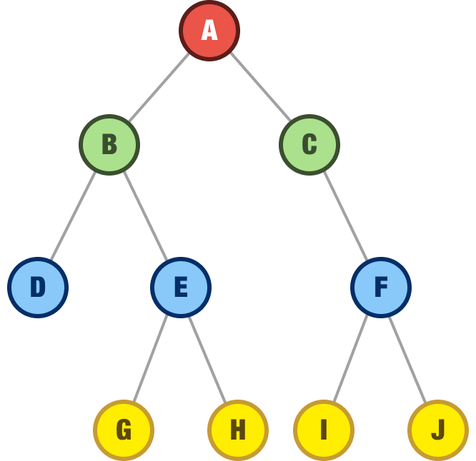
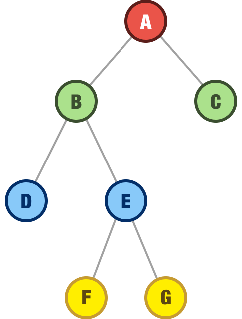
A binary tree, on the surface, looks just like a boring regular tree that allows us to store data in a hierarchical manner. Below is an example of what a binary tree looks like:

What makes binary trees different is that, unlike regular trees where anything goes, we have three strict rules our tree must adhere to in order to be classified as a binary tree. The rules are:

1. Each node can only have 0, 1, or 2 children
2. The tree can only have a single root node
3. There can be only one path to a node from the root

Let's dive a bit deeper into these rules, for they are important to understand. They will help explain why the binary tree works the way it does, and it sets us up for learning about other tree variants, such as the binary search tree next.

Rules Explained

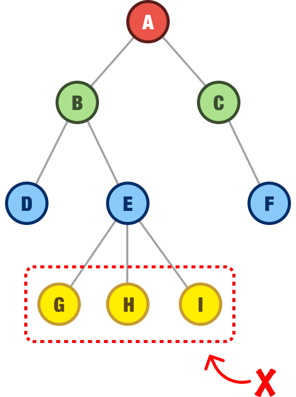
The first rule is that each node in a binary tree can only have 0, 1, or 2 children. If a node happens to have more than two children, that’s a problem:

The second rule is that a binary tree must have only a single root node:

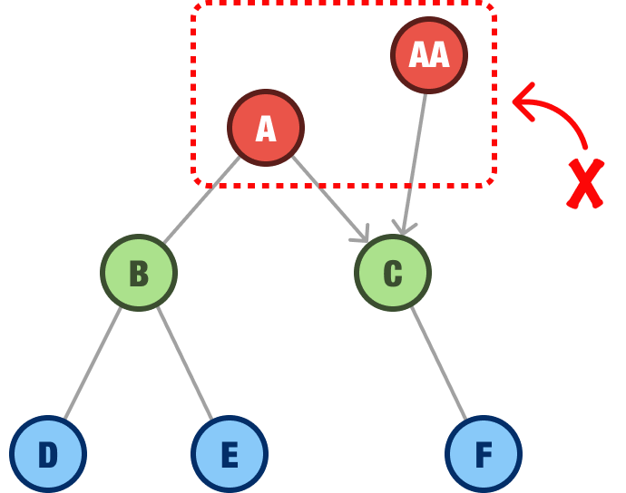
In this example, we have both the A node and the AA node competing for who gets to be the primary root. While multiple root nodes is acceptable in certain other tree-based data structures, they aren’t allowed for binary trees.

Now, we get to the last rule. The last rule is that there can be only one path from the root to any node in the tree:

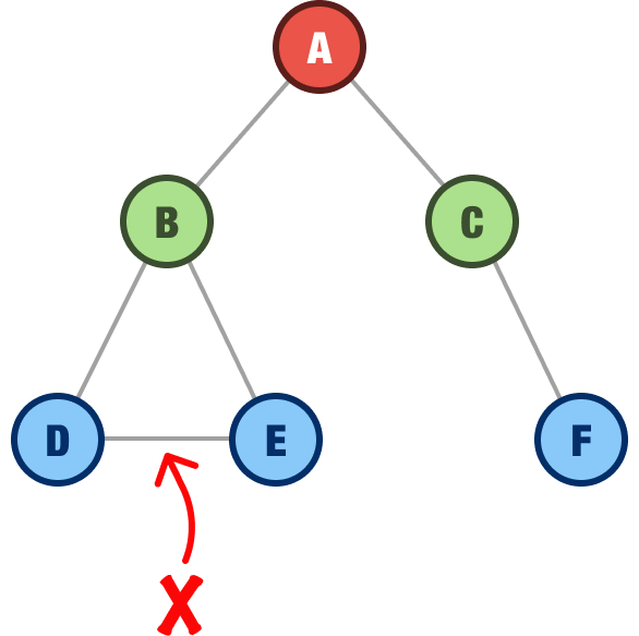
As we can see in this example, using node D as our destination, we can get there in two ways from our root. One way is by A - B - D. The other way is by A - B - E - D. We can’t have that and call ourselves a binary tree.

Binary Tree Variants

Binary trees, even with their stricter rules, appear in a handful of popular variants. These variants play a large role in how well our friendly binary tree performs at common data operations, how much space it takes up, and more. For now, we’ll avoid the math and focus on the high-level details.

Full Binary Tree

The full binary tree, sometimes referred to as either a strict binary tree or proper binary tree, is a tree where all non-leaf nodes have their full two children:

In this example, we can see that the non-leaf nodes A, B, and E all have two children.

Complete Binary Tree

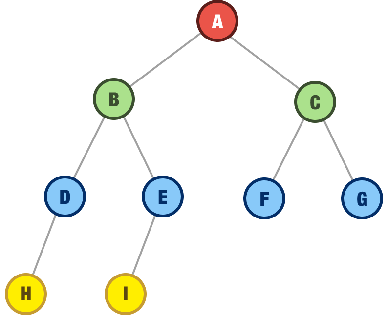
A complete binary tree is one where all rows of the nodes are filled (where each parent has two children) except for the last row of nodes:

For this last row, there are some rules on how the nodes should appear. If the last row has any nodes, those nodes need to be filled continuously, starting from the left with no gaps. This wouldn’t be acceptable, for example:

There is a gap where the D node is missing its right child, so we weren’t continuously filling in the last row of nodes from the left.

Perfect Binary Tree

A perfect binary tree is a binary tree where every level of the tree is fully filled with nodes:

As a consequence of that requirement, all the leaf nodes are also at the same level.

Balanced Binary Tree
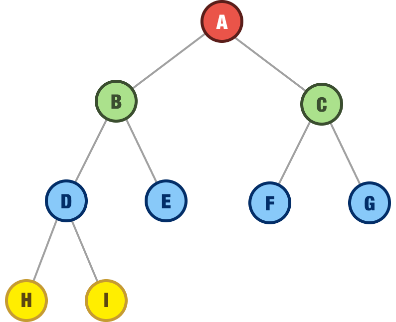
A balanced binary tree is a binary tree in which the height of the left and right subtrees of each node is not more than one apart. Below is an example of a balanced binary tree:

In other words, this means that the tree is not lopsided. All nodes can be accessed efficiently.

Degenerate Binary Tree

In a degenerate binary tree, each parent node has only one child node:

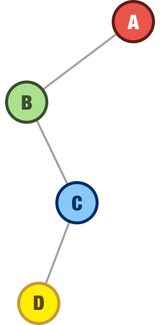
This means that the tree is essentially a linear data structure, like an array, with all nodes connected in a single path. Any advantages a tree-like structure provides are lost here, hence the degenerate classifier.

What about Adding, Removing, and Finding Nodes?

As with any data structure, a common operation for us will be to add nodes, remove nodes, or find a particular node we are looking for. To echo a point I made earlier, binary trees in their generic state are not very efficient data structures. Learning how to perform common operations on them may be helpful from a general knowledge-gathering exercise, but they won’t be too helpful in real-world situations. Instead of covering something that you will rarely benefit from, I’m going to put a pin on this topic and cover this in more detail as part of looking at a more efficient implementation of the binary tree, the binary search tree, later.

A Simple Binary Tree Implementation

Before we wrap things up, let’s look at a simple binary tree implementation. The star of our implementation is going to be the node, and here is how we will represent this in JavaScript:

class Node {
  constructor(data) {
    this.data = data;
    this.left = null;
    this.right = null;
  }
}

We have a Node class, and it takes a data value as its argument, which it stores as a property called data on itself. Our node also stores two additional properties for left and right.

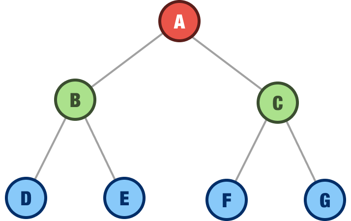
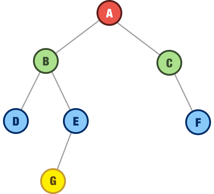
Let’s re-create the following binary tree using what we have:

The full code for re-creating this using our Node class will look as follows:

class Node {
  constructor(data) {
    this.data = data;
    this.left = null;
    this.right = null;
  }
}

const rootNodeA = new Node("A");
const nodeB = new Node("B");
const nodeC = new Node("C");
const nodeD = new Node("D");
const nodeE = new Node("E");
const nodeF = new Node("F");
const nodeG = new Node("G");

rootNodeA.left = nodeB;
rootNodeA.right = nodeC;

nodeB.left = nodeD;
nodeB.right = nodeE;

nodeE.left = nodeF;
nodeE.right = nodeG;

Notice that we are creating a new Node object for each node in our tree, and the argument we pass in to the constructor is the letter value of each node:

const rootNodeA = new Node("A");
const nodeB = new Node("B");
const nodeC = new Node("C");
const nodeD = new Node("D");
const nodeE = new Node("E");
const nodeF = new Node("F");
const nodeG = new Node("G");

Our implementation of the Node object will support data ranging from simple (such as a letter) to overly complex. In some cases, our nodes will be made up of numbers. In other cases, our nodes will be made up of complex objects. We’ll look at some more elaborate examples in the future.

Once we have our nodes created, we set each node’s left and right properties to the corresponding child node:

rootNodeA.left = nodeB;
rootNodeA.right = nodeC;

nodeB.left = nodeD;
nodeB.right = nodeE;

nodeE.left = nodeF;
nodeE.right = nodeG;

If a node happens to be a leaf node, we don’t do anything extra. It is safe to say that if a node doesn’t have anything set for its left or right property, it is a leaf. It has no children.

Conclusion

In the many past sections, through lots of words and countless diagrams, we learned about binary trees! The 411 is that a binary tree is a data structure that consists of nodes with an important constraint: each node can have at most two child nodes. The unique constraint of the binary tree allows us to use them to efficiently search, sort, and store data. Now, we didn't cover any of that here. The reason is that a binary tree by itself is too generic. The more useful variant of the binary tree is the binary search tree, and we are going to look at it next.

Just a final word before we wrap up. If you have a question and/or want to be part of a friendly, collaborative community of over 220k other developers like yourself, post on the forums for a quick response!