by kirupa |
13 January 2006In the
previous page, you received a
brief introduction to searching and how
our search tree will be defined. In this page, I demonstrate how Depth First
Search works.
Depth First Search
Depth first search works by taking a node, checking its neighbors, expanding
the first node it finds among the neighbors, checking if that expanded node is
our destination, and if not, continue exploring more nodes.
The above explanation is probably confusing if this is your
first exposure to depth first search. I hope the following demonstration will
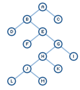
help more. Using our same search tree, let's find a path between nodes A and F:

Step 0
Let's start with our root/goal node:

I will be using two lists to keep track of what we are doing -
an Open list and a Closed List. An Open list keeps track of what
you need to do, and the Closed List keeps track of what you have already done. Right now, we only have our starting
point, node A. We haven't done anything to it yet, so let's add it to our
Open list.
-
Open List: A
-
Closed List: <empty>
Step 1
Now, let's explore the neighbors of our A node. To put another way, let's take
the first item from our Open list and explore its neighbors:

Node A's neighbors are the B and C nodes. Because we are now
done with our A node, we can remove it from our Open list and add it to our
Closed List. You aren't done with this step though. You now have two new nodes B
and C that need exploring. Add those two nodes to our Open list.
Our current Open and Closed Lists contain the following data:
-
Open List: B, C
-
Closed List: A
Step 2
Our Open list contains two items. For depth first search and breadth first
search, you always explore explore
the first item from our Open list. The first item in our Open list is the B node.
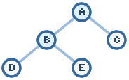
B is not our destination, so let's explore its neighbors:

Because I have now expanded B, I am going to remove it from
the Open list and add it to the Closed List. Our new nodes are D and E, and we add
these nodes to the beginning of our Open list:
-
Open List: D, E, C
-
Closed List: A, B
Step 3
You should start to see a pattern forming. Because D is at the beginning of our
Open List, we expand it. D isn't our destination, and it does not contain any neighbors.
All you do in
this step is remove D from our Open List and add it to our Closed List:
-
Open List: E, C
-
Closed List: A, B, D
Step 4
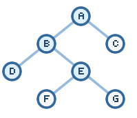
We now expand the E node from our Open list. E is not our destination, so we
explore its neighbors and find out that it contains the neighbors F and G.
Remember, F is our target, but we don't stop here though. Despite F being on our path, we only end when we are about to expand our
target Node - F in this case:

Our Open list will have the E node removed and
the F and G nodes added. The removed E node will be added to our Closed List:
-
Open List: F, G, C
-
Closed List: A, B, D, E
Step 5
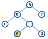
We now expand the F node. Since it is our intended destination, we stop:

We remove F from our Open list and add it to our
Closed List. Since we are at our destination, there is no need to expand F in
order to find its neighbors. Our final Open and Closed Lists contain the
following data:
-
Open List: G, C
-
Closed List: A, B, D, E, F
The final path taken by our depth first search
method is what the final value of our Closed List is: A, B, D, E, F. Towards the
end of this tutorial, I will analyze these results in greater detail so that you
have a better understanding of this search method.
On the next page, let's learn how breadth first
search would work.
Onwards to the next page!
|